21Case Study: Business Analytics and Customer Insights
21.1 Introduction: AutoML and Automated Feature Engineering for Customer Insight
Across the previous chapters, we developed a descriptive analytical toolkit that moves from exploratory association analysis through segmentation to interpretable model summaries and communication. This case study applies the final two layers of that toolkit to a business setting: automated feature engineering, which structures the search for informative derived predictors, and AutoML-style model comparison, which surveys multiple model families under a common evaluation protocol.
The analytical emphasis is intentionally non-predictive. In business analytics, the goal is often to understand which customer behaviors drive value heterogeneity and how they interact, not to optimize a prediction system. AutoML and automated feature engineering support this by making the search process explicit and transparent rather than driven by ad hoc choices. They allow us to document what the data supports across a range of model families and feature representations, rather than committing to a single handcrafted specification.
21.2 Business Context and Customer Analytics Questions
We analyze a subscription business with recurring transaction data. The analytical questions we address are:
How do customer transaction patterns vary across segments?
Which transformation and interaction terms most improve our understanding of customer value, according to a systematic candidate screening procedure (following Chapter 18)?
How does a multi-model AutoML comparison reveal which model family best captures customer value structure (following Chapter 17)?
What interpretable customer profiles emerge from variable importance rankings?
How can we communicate customer insights to product and marketing teams?
21.3 Customer Data and Baseline Profiling
We construct a customer dataset from transaction-level data aggregated to customer level. For reproducibility, we simulate transaction data that reflects realistic e-commerce patterns.
set.seed(789)n_customers <-500customer_transactions <-expand_grid(customer_id =1:n_customers,month =1:12) |>mutate(n_trans =rpois(n(), lambda =2+rnorm(n(), mean =0, sd =0.5)) +1,avg_transaction_value =runif(n(), min =20, max =200),trans_amount = n_trans * avg_transaction_value ) |>slice_sample(prop =0.7)nrow(customer_transactions)
[1] 4200
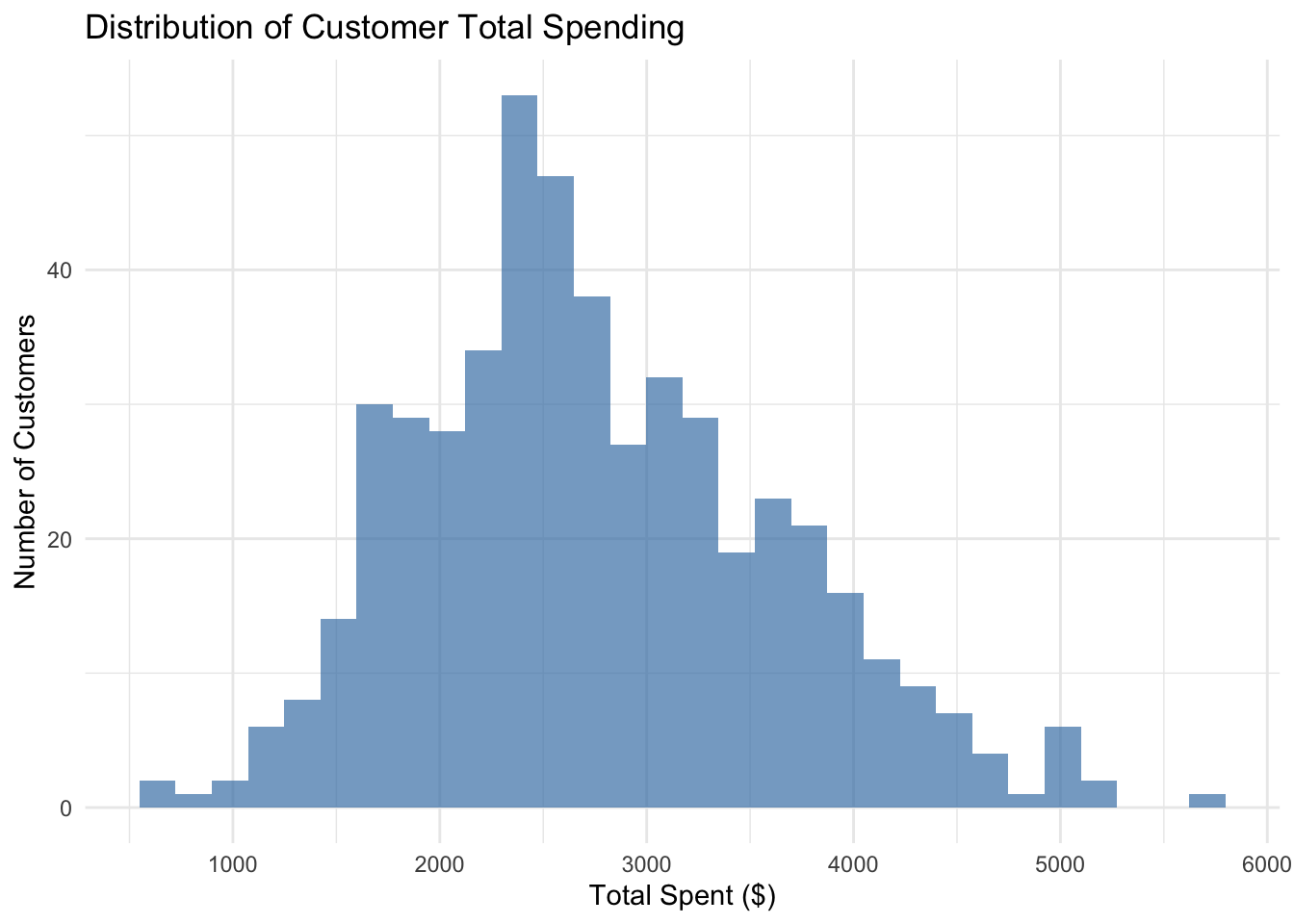
From transaction data, we aggregate to customer-level metrics that serve as both features and communication targets.
customer_base |>ggplot(aes(x = total_spent)) +geom_histogram(fill ="steelblue", alpha =0.7) +labs(title ="Distribution of Customer Total Spending",x ="Total Spent ($)",y ="Number of Customers" ) +theme_minimal()
21.4 RFM-Style Baseline Segmentation
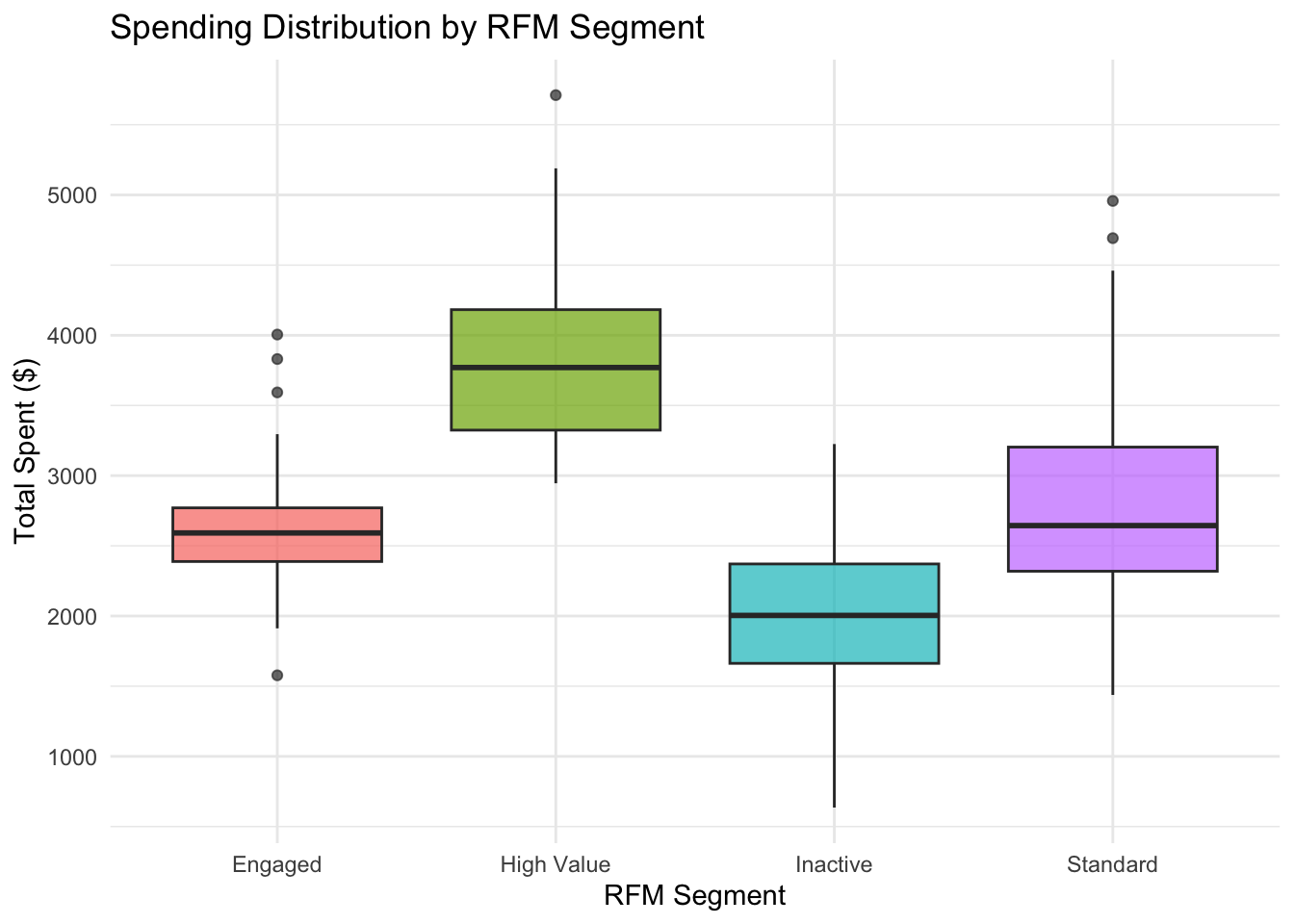
Before automated methods, we create a simple baseline segmentation based on RFM, a widely used customer analytics framework: Recency (how recently customers bought), Frequency (how often they buy), and Monetary value (how much they spend). We use months_active as a proxy for recency, n_transactions for frequency, and total_spent for monetary value. We create quintile-based scores for each dimension and define 4 segments based on combinations of these scores.
rfm_segments |>ggplot(aes(x = rfm_segment, y = total_spent, fill = rfm_segment)) +geom_boxplot(alpha =0.7) +labs(title ="Spending Distribution by RFM Segment",x ="RFM Segment",y ="Total Spent ($)",fill ="Segment" ) +theme_minimal() +theme(legend.position ="none")
This baseline segmentation provides a business-interpretable starting point. The automated feature engineering and model search steps that follow will reveal whether richer representations of customer behavior capture meaningful additional structure.
21.5 Automated Feature Engineering with Candidate Screening
RFM is an effective summary, but it discards information about the shape of customer behavior. Automated feature engineering, following the workflow developed in Chapter 18, provides a principled alternative: rather than manually selecting derived features, we generate a library of candidate transformations and interaction terms, then screen them by cross-validated predictive improvement.
We reserve a held-out test set before any screening, following the same separation used in Chapter 18.
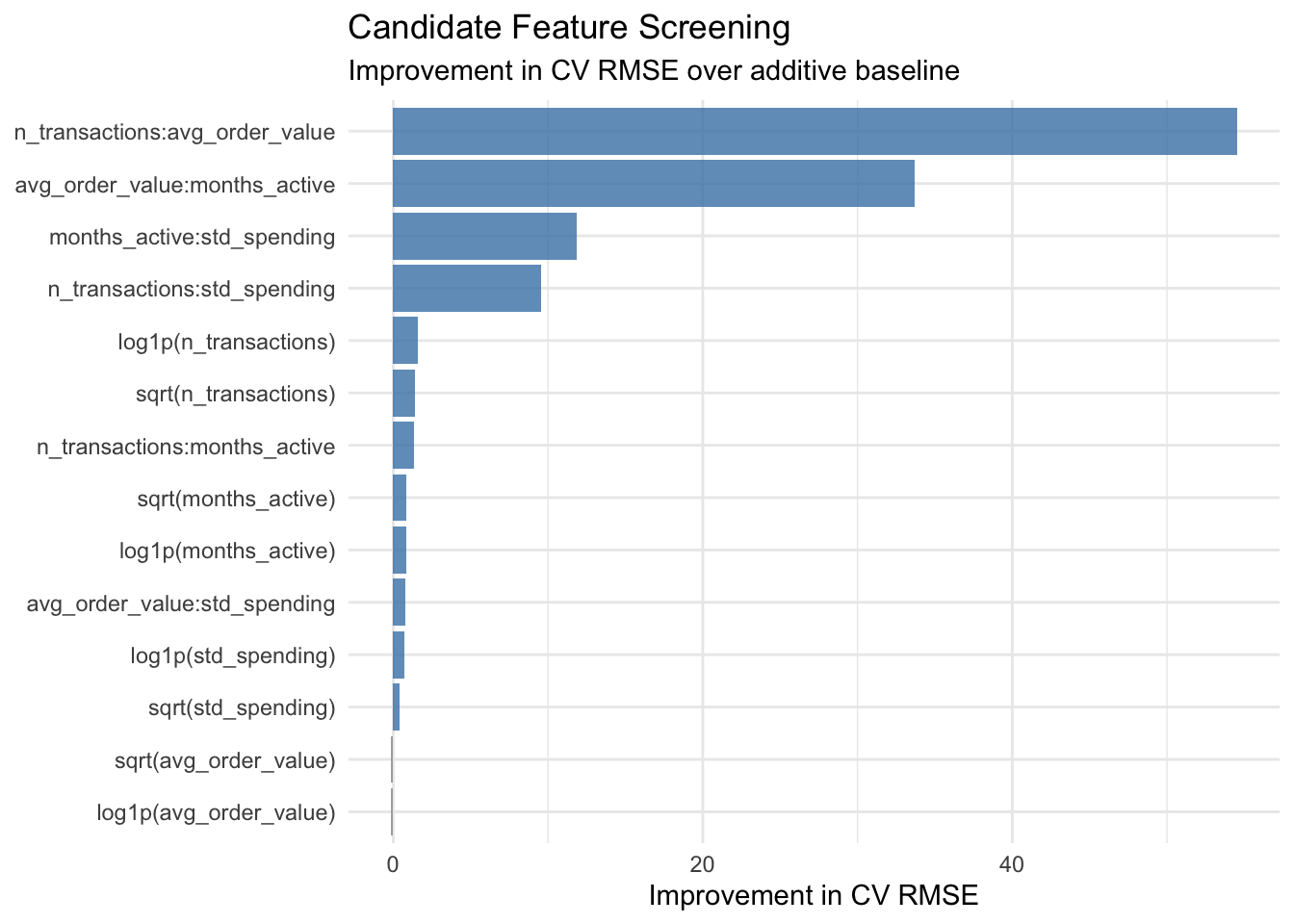
We define four raw features and generate two classes of candidate terms: element-wise transformations (log and square root, which are useful for right-skewed customer metrics) and pairwise interactions (which capture how feature combinations relate to spending).
We define a baseline additive linear model and evaluate each candidate term by augmenting this baseline with one additional feature at a time. The evaluation uses five-fold cross-validation on the analysis set, with holdout RMSE as the criterion.
rmse <-function(actual, predicted) {sqrt(mean((actual - predicted)^2))}make_folds <-function(n, k =5, seed =123) {set.seed(seed)sample(rep(seq_len(k), length.out = n))}cv_rmse_lm <-function(data, formula_obj, fold_id) { k <-length(unique(fold_id)) fold_errors <-numeric(k)for (fold inseq_len(k)) { train_fold <- data[fold_id != fold, , drop =FALSE] valid_fold <- data[fold_id == fold, , drop =FALSE] fit <-lm(formula_obj, data = train_fold) pred <-as.numeric(predict(fit, newdata = valid_fold)) fold_errors[fold] <-rmse(valid_fold[["total_spent"]], pred) }mean(fold_errors)}fold_id <-make_folds(n =nrow(analysis_data), k =5, seed =456)baseline_formula <- total_spent ~ n_transactions + avg_order_value + months_active + std_spendingbaseline_cv <-cv_rmse_lm(analysis_data, baseline_formula, fold_id)cat("Baseline CV RMSE:", round(baseline_cv, 2), "\n")
The screening leaderboard shows which feature representations add descriptive value beyond the additive baseline. Interaction terms that appear at the top reflect genuine behavioral coupling between customer metrics: for example, a high-frequency customer with a high average order value represents a qualitatively different profile from one where only one dimension is elevated. This kind of multiplicative structure is not captured by the additive baseline and is exactly the type of pattern that automated feature engineering helps surface.
It is worth noting a methodological point: some interaction candidates may show strong improvement partly because of the mathematical construction of the data. In practice, a business analyst should inspect top-ranked features carefully to distinguish between genuine behavioral insights and artefacts of variable construction.
21.6 AutoML-Style Model Search and Leaderboard
Automated feature engineering answers the question of what to include as inputs. An AutoML model search, following Chapter 17, answers the complementary question: which model family best captures the structure of customer value heterogeneity across those inputs?
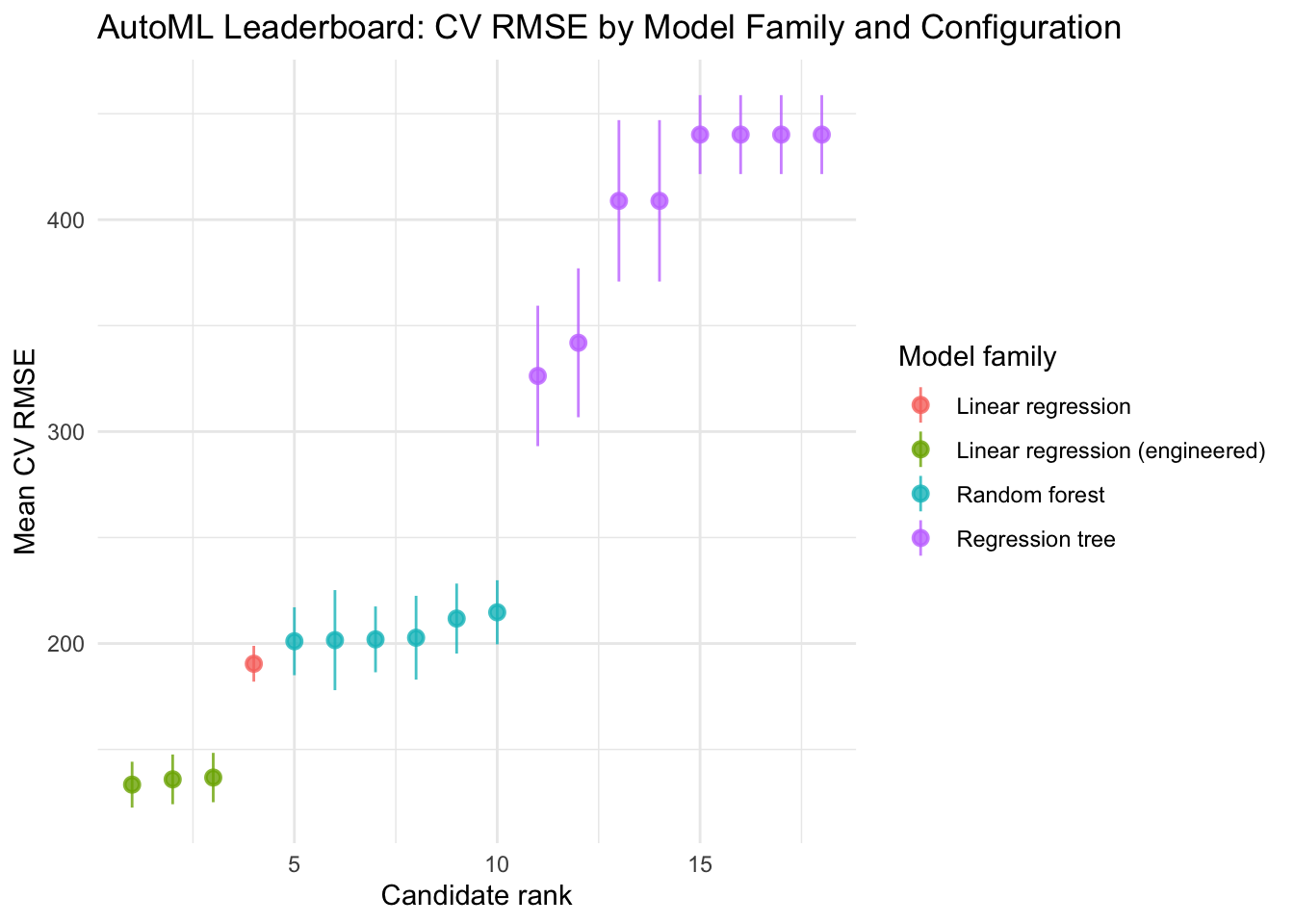
We compare three model families under a common five-fold cross-validation protocol: a linear regression baseline, regression trees with several hyperparameter configurations, and random forests with several mtry values. This mirrors the search structure developed in Chapter 17, applied to the customer data.
automl_leaderboard |>mutate(rank =seq_len(n())) |>ggplot(aes(x = rank, y = mean_rmse, color = family,ymin = mean_rmse - sd_rmse, ymax = mean_rmse + sd_rmse)) +geom_pointrange(alpha =0.8) +labs(title ="AutoML Leaderboard: CV RMSE by Model Family and Configuration",x ="Candidate rank",y ="Mean CV RMSE",color ="Model family" ) +theme_minimal()
The leaderboard now spans four model families: the plain linear baseline, linear regression augmented with top screened features from the previous section, regression trees, and random forests. This is the natural combination of the feature engineering workflow (Chapter 18) and the model search workflow (Chapter 17): screening candidates first and then searching over model families that include those candidates.
The leaderboard identifies the winning configuration, both in terms of model family and feature representation, under a common evaluation protocol. If a plain linear model with raw features wins, the relationship is additive and no engineered features are needed. If an augmented linear model wins, the interaction or transformation terms improve things but complex nonlinear models do not. If ensemble models win, there is genuine nonlinear or interaction structure that linear representations cannot capture regardless of feature engineering.
Comparing the winning CV RMSE back to the baseline (plain linear regression, evaluated in the same folds) provides a calibrated sense of how much the combined feature engineering and model search workflow gained over the starting point.
The winning model, linear model augmented with the top 3 features, is used for all downstream analysis.
21.7 Feature Importance and Variable Selection
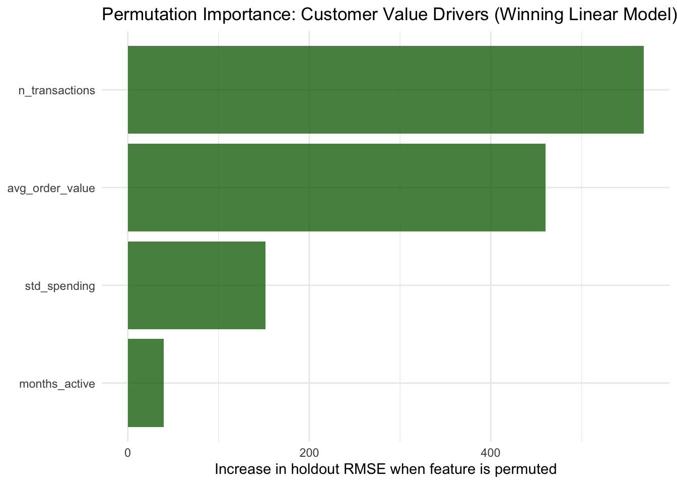
We fit the winning model on the full analysis set and rank the original raw predictors by model-agnostic permutation importance, following Chapter 14. Permutation importance is computed by measuring how much holdout RMSE increases when each feature is randomly shuffled, breaking its relationship with the outcome while leaving the model unchanged. A large increase signals a feature the model relies on heavily; a near-zero increase signals that the model can predict almost as well without it.
Permuting a raw feature (for example n_transactions) affects all formula terms that depend on it, including any engineered terms such as log1p(n_transactions) or interaction terms. This means the importance scores correctly attribute signal to the original customer behavior variables rather than to their derived representations, regardless of which formula won the leaderboard.
# Recover the formula of the best linear model from the registrywinner_key <-paste(automl_leaderboard$family[1], automl_leaderboard$config[1], sep ="||")winning_formula <-if (!is.null(formula_registry[[winner_key]])) { formula_registry[[winner_key]]} else { automl_formula # fallback: plain baseline}lm_final <-lm(winning_formula, data = analysis_data)cat("Winning formula:\n")
importance_tbl |>ggplot(aes(x =reorder(feature, importance), y = importance)) +geom_col(fill ="darkgreen", alpha =0.75) +coord_flip() +labs(title ="Permutation Importance: Customer Value Drivers (Winning Linear Model)",x =NULL,y ="Increase in holdout RMSE when feature is permuted" ) +theme_minimal()
Cross-referencing importance rankings with the feature screening leaderboard provides a consistency check. When the same predictors appear both as top candidates in the screening step and as high-importance variables in the winning model, there is convergent evidence that these features carry genuine descriptive signal. When rankings differ, the discrepancy may reflect collinearity between predictors or sensitivity to how the candidate term interacts with the baseline model form.
21.8 Customer Targeting and Segmentation
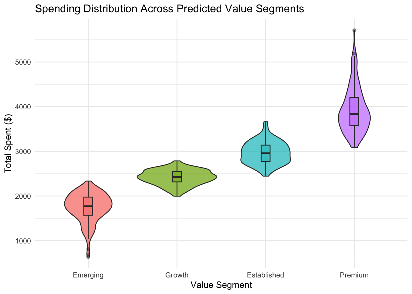
Using the trained model, we score all customers and partition them by predicted value into four business-relevant tiers.
customer_scored |>ggplot(aes(x = value_segment, y = total_spent, fill = value_segment)) +geom_violin(alpha =0.7) +geom_boxplot(width =0.1, alpha =0.5) +labs(title ="Spending Distribution Across Predicted Value Segments",x ="Value Segment",y ="Total Spent ($)",fill ="Segment" ) +theme_minimal() +theme(legend.position ="none")
These data-driven segments can inform differentiated marketing, pricing, or retention strategies. The model-based partitioning complements the rule-based RFM segmentation from earlier in the chapter: the two approaches can be compared directly to examine whether the automated method adds resolution beyond the manual baseline.
21.9 Communicating Customer Insights to Business Stakeholders
Data-driven customer segmentation is most valuable when translated into actionable business narratives. The following insights bridge the feature screening and AutoML results with business language.
Insight 1: Transaction frequency and average order value are the primary value drivers. Permutation importance indicates that n_transactions and avg_order_value are the two strongest contributors to predicted customer spending. The feature screening step confirms that their interaction term provides additional explanatory power beyond either predictor in isolation. This suggests that growth actions should target basket expansion (higher order value) and repeat purchase behavior (higher transaction volume) simultaneously, rather than treating them as independent levers.
Insight 2: Customer value is well described by an additive linear model, complexity is not required. The AutoML leaderboard shows that linear regression outperforms all tree-based and ensemble alternatives. This is a substantive finding: it means that the drivers of total spending combine approximately additively, and a linear combination of transaction frequency, order value, tenure, and spending variability captures the main patterns. For business planning, this simplicity is an asset: additive contributions are directly interpretable as marginal value drivers without requiring complex model explanations.
Insight 3: A four-tier segmentation is operationally useful. The model separates customers into four value tiers with rising average spend from one tier to the next. Each tier can receive a different plan, for instance: low-cost activation for Emerging, frequency-building offers for Growth, loyalty reinforcement for Established, and high-touch retention for Premium. The feature importance rankings also give each tier a behavioral profile that supports message targeting within that tier.
These insights translate feature rankings and model structure into business language that can guide strategy without requiring stakeholders to engage with the underlying algorithmic details.
21.10 Holdout Validation and Model Performance
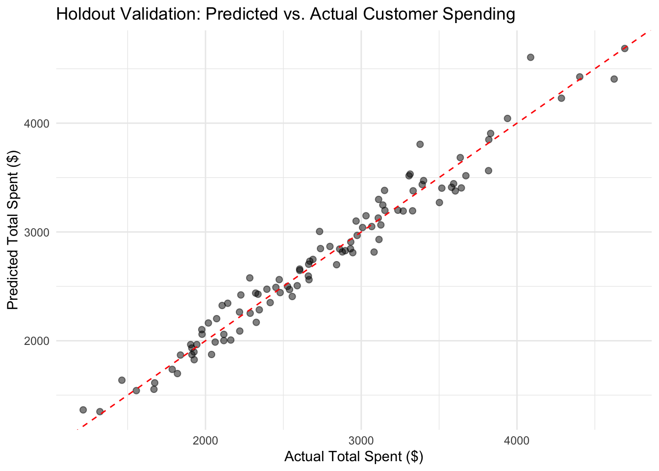
To assess whether the segmentation generalizes beyond the analysis sample, we evaluate model performance on the held-out test set reserved at the start of the analysis.
tibble::tibble(actual = test_data$total_spent,predicted = test_pred) |>ggplot(aes(x = actual, y = predicted)) +geom_point(alpha =0.5, size =2) +geom_abline(intercept =0, slope =1, color ="red", linetype ="dashed") +labs(title ="Holdout Validation: Predicted vs. Actual Customer Spending",x ="Actual Total Spent ($)",y ="Predicted Total Spent ($)" ) +theme_minimal()
Holdout performance confirms that the model’s segmentation and feature ranking reflect stable patterns in customer behavior. Comparing CV RMSE from the leaderboard to the holdout RMSE provides a consistency check: a large discrepancy would suggest over-optimistic leaderboard estimates, possibly due to overfitting during the feature screening or model search phase.
21.11 Limitations and Reproducibility Notes
Several caveats warrant attention.
This case study uses simulated data. Real customer data often contains temporal autocorrelation, seasonality, sparse records, and missing values that require additional preprocessing. The feature-outcome relationships illustrated here are deliberately simple to make the workflow visible.
The strong contribution of the interaction between n_transactions and avg_order_value in the feature screening partly reflects the mathematical construction of total_spent in this dataset. In applied settings, careful examination of whether top-ranked features encode genuine behavioral insight or are artefacts of variable construction is essential.
The AutoML search is intentionally lightweight. Production systems would explore larger candidate spaces, use repeated cross-validation, and apply model-specific regularization. The principles remain the same, but the engineering budget is different.
Feature importance can be sensitive to feature correlation and scale. When predictors are correlated, importance scores should be interpreted as group-level signals rather than individual contributions.
All random components use set seeds for reproducibility. In applied settings, stability checks across alternative model specifications and multiple random seeds are recommended before using results to inform strategic decisions.
21.12 Summary and Key Takeaways
Automated feature engineering systematizes the search for informative derived predictors by generating a candidate library and screening it by cross-validated improvement, following the workflow from Chapter 18.
AutoML-style model comparison surveys multiple model families under a common evaluation protocol, producing a leaderboard that describes how much structure different algorithms can extract from the data, following Chapter 17.
The combination of feature screening and model leaderboard provides two complementary views of the same question: what drives customer value, and how complex is that structure?
Model-agnostic permutation importance applied to the winning model translates AutoML and feature engineering results into a ranked list of customer behavior drivers, regardless of which model family prevailed.
Data-driven customer segmentation supports differentiated targeting and resource allocation.
The emphasis throughout is descriptive: AutoML and automated feature engineering are instruments for learning about data, not for deploying prediction systems.
21.13 Looking Ahead
This case study focused on automated feature engineering and AutoML-style model comparison as descriptive instruments for customer insight. The next chapter consolidates the core lessons from all three case studies (policy, health, and business), highlights the main practical principles of descriptive tabular analysis, and closes with recommendations for applying this workflow responsibly in real-world projects.