data(Boston, package = "MASS")

set.seed(123)
idx <- sample(seq_len(nrow(Boston)), size = 0.7 * nrow(Boston))
train <- Boston[idx, ]
test <- Boston[-idx, ]

predictors <- c("lstat", "rm", "ptratio", "indus", "nox", "crim")
formula <- as.formula(paste("medv ~", paste(predictors, collapse = " + ")))
mtry_reg <- length(attr(terms(formula), "term.labels"))12 Ensemble Methods as Descriptive Instruments
12.1 Introduction: From Single Trees to Ensembles
The previous two chapters introduced regression and classification trees as transparent tools for segmentation. They are appealing precisely because they are easy to read, but in some cases they may also be unstable. For instance, small changes in the data can lead to different splits and different segment definitions. Ensemble methods respond to that instability by combining many trees into a single model. The result is often more accurate and more stable, at the cost of some immediacy in interpretation.
In a descriptive workflow, ensembles can still be valuable. They provide robust summaries of variable influence and a smoother picture of how predictors shape outcomes. We can treat them as instruments for stabilizing patterns that appear in single trees, rather than as black boxes that replace interpretive judgment.
This chapter introduces three ensemble ideas that are central in practice: bagging, random forests, and gradient boosting. We focus on their descriptive roles, how they average or accumulate information, and how we can extract interpretable summaries from them.
12.2 Why Ensembling Helps
Ensemble methods rest on a simple principle. If we fit many models that are each somewhat noisy, then averaging them can reduce variance. For tree based models, this is especially important because recursive partitioning is high variance by construction. Even a single split can change if one observation is perturbed.
From a descriptive standpoint, the key idea is that repeated tree fitting can help identify consistent signals. Rather than trusting one tree, we can look at patterns that persist across many resamples. Variable importance and partial dependence are two common summaries, and we will return to them in later chapters.
12.3 Bagging: Bootstrap Aggregation
Bagging, short for bootstrap aggregation, is the simplest ensemble approach (Breiman 1996). We take many bootstrap samples of the data, fit a tree on each sample, and average their predictions. For regression, we average predicted values. For classification, we average class probabilities and then choose a class if needed.
Bagging reduces variance because each tree is fitted on a slightly different dataset. A useful side benefit is the out of bag (OOB) observations, the roughly one third of data points not included in each bootstrap sample. By predicting those points, we obtain a built in estimate of predictive error without a separate validation set.
12.5 Gradient Boosting: Sequential Refinement
Boosting combines trees in a different way (Friedman 2001). Instead of building trees independently and averaging them, boosting builds trees sequentially. Each new tree is trained to predict the residuals of the current model, so the ensemble gradually improves its fit.
Gradient boosting can be seen as an additive model of many small trees. For descriptive analysis, this can be attractive because it yields smooth, flexible fits while still allowing us to inspect variable importance and functional relationships. However, the model is more complex, so interpretability depends heavily on the summaries we choose to extract.
12.6 A Reproducible Example with Housing Prices
We return to the Boston housing data. The outcome is medv, and we use a modest set of predictors. We will compare a single regression tree, a bagged tree ensemble, a random forest, and a gradient boosted model using a simple train test split.
12.6.1 A Single Regression Tree
We begin with a tree as a baseline. The goal is not to optimize hyperparameters, but to provide a comparable reference for the ensemble models.
set.seed(123)
tree_fit <- rpart(
    formula,
    data = train,
    method = "anova",
    control = rpart.control(minsplit = 30, cp = 0.001)
)

tree_pred <- predict(tree_fit, newdata = test)
tree_rmse <- sqrt(mean((test$medv - tree_pred)^2))

tree_rmse
[1] 4.677431RMSE, the root mean squared error, summarizes the typical prediction error by taking the square root of the average squared difference between observed and predicted values. It is expressed in the same units as medv, so smaller values indicate closer fit to the observed housing prices.
12.6.2 Bagging and Random Forests
Bagging is equivalent to a random forest where all predictors are considered at each split. We fit both bagging and a standard random forest to compare their behavior.
set.seed(123)
bag_fit <- randomForest(
    formula,
    data = train,
    mtry = mtry_reg,
    ntree = 500,
    importance = TRUE
)

rf_fit <- randomForest(
    formula,
    data = train,
    mtry = max(1, floor(mtry_reg / 3)),
    ntree = 500,
    importance = TRUE
)

bag_pred <- predict(bag_fit, newdata = test)
rf_pred <- predict(rf_fit, newdata = test)

bag_rmse <- sqrt(mean((test$medv - bag_pred)^2))
rf_rmse <- sqrt(mean((test$medv - rf_pred)^2))

bag_rmse
[1] 3.93907rf_rmse[1] 3.55459912.6.3 Gradient Boosting
For boosting we use a standard configuration with shallow trees and a small learning rate. The number of trees is selected by cross validation within the gbm routine.
set.seed(123)
gbm_fit <- gbm(
    formula,
    data = train,
    distribution = "gaussian",
    n.trees = 2000,
    interaction.depth = 3,
    shrinkage = 0.01,
    bag.fraction = 0.7,
    cv.folds = 5,
    verbose = FALSE
)

best_iter <- gbm.perf(gbm_fit, method = "cv", plot.it = FALSE)
gbm_pred <- predict(gbm_fit, newdata = test, n.trees = best_iter)
gbm_rmse <- sqrt(mean((test$medv - gbm_pred)^2))

best_iter
[1] 1990gbm_rmse[1] 3.8882612.6.4 Comparing Errors
We summarize the test set RMSE values. The exact numbers depend on the split, but the pattern is often consistent, ensembles tend to outperform a single tree in predictive accuracy.
rmse_tbl <- tibble::tibble(
    Model = c("Single tree", "Bagging", "Random forest", "Gradient boosting"),
    RMSE = c(tree_rmse, bag_rmse, rf_rmse, gbm_rmse)
)

rmse_tbl |>
    gt() |>
fmt_number(columns = RMSE, decimals = 3)| Model | RMSE |
|---|---|
| Single tree | 4.677 |
| Bagging | 3.939 |
| Random forest | 3.555 |
| Gradient boosting | 3.888 |
When we compare the four RMSE values, we read them as competing summaries of average prediction error on the same test data. A lower RMSE indicates that the model, on average, is closer to observed values. If the ensemble models show smaller RMSE than the single tree, this supports the idea that averaging or sequential refinement reduces variance and improves accuracy. Differences that are small relative to the outcome scale are still worth noting, but they may not imply large substantive gains, so it is helpful to interpret them alongside descriptive goals rather than only as a ranking.
With that regression baseline in place, we now shift to a binary outcome to see how the same ensemble ideas translate to classification.
12.7 A Classification Example: Pima Diabetes
Ensembles are equally useful when the outcome is categorical. We use the Pima diabetes data from MASS. The outcome indicates diabetes status, and the predictors are clinical measurements. We use the provided training and test splits and repeat the same ensemble comparisons. A common summary is accuracy, the proportion of cases assigned to the correct class, but we also inspect a confusion matrix and macro averaged precision and recall to account for class imbalance.
data(Pima.tr, package = "MASS")
data(Pima.te, package = "MASS")

train_pima <- Pima.tr
test_pima <- Pima.te

pima_formula <- type ~ npreg + glu + bp + skin + bmi + ped + age
mtry_pima <- length(attr(terms(pima_formula), "term.labels"))
12.7.1 A Single Classification Tree
We begin with a single classification tree as a baseline, comparable to the regression tree in the Boston example.
set.seed(123)
pima_tree_fit <- rpart(
    pima_formula,
    data = train_pima,
    method = "class",
    control = rpart.control(minsplit = 20, cp = 0.01)
)

pima_tree_pred <- predict(pima_tree_fit, newdata = test_pima, type = "class")
pima_tree_acc <- mean(pima_tree_pred == test_pima$type)

pima_tree_acc
[1] 0.731927712.7.2 Ensemble Methods for Classification
Now we fit the three ensemble methods for comparison.
set.seed(123)
pima_bag <- randomForest(
    pima_formula,
    data = train_pima,
    mtry = mtry_pima,
    ntree = 500
)

pima_rf <- randomForest(
    pima_formula,
    data = train_pima,
    mtry = max(1, floor(mtry_pima / 2)),
    ntree = 500,
    importance = TRUE
)

pima_bag_pred <- predict(pima_bag, newdata = test_pima, type = "class")
pima_rf_pred <- predict(pima_rf, newdata = test_pima, type = "class")

pima_bag_acc <- mean(pima_bag_pred == test_pima$type)
pima_rf_acc <- mean(pima_rf_pred == test_pima$type)

set.seed(123)
pima_gbm <- gbm(
    type_num ~ npreg + glu + bp + skin + bmi + ped + age,
    data = train_pima |> mutate(type_num = ifelse(type == "Yes", 1, 0)),
    distribution = "bernoulli",
    n.trees = 1500,
    interaction.depth = 2,
    shrinkage = 0.05,
    bag.fraction = 0.7,
    cv.folds = 5,
    verbose = FALSE
)

pima_best <- gbm.perf(pima_gbm, method = "cv", plot.it = FALSE)
pima_prob <- predict(pima_gbm, newdata = test_pima, n.trees = pima_best, type = "response")
pima_gbm_pred <- ifelse(pima_prob > 0.5, "Yes", "No")
pima_gbm_pred <- factor(pima_gbm_pred, levels = levels(test_pima$type))

pima_gbm_acc <- mean(pima_gbm_pred == test_pima$type)

pima_bag_acc
[1] 0.75pima_rf_acc[1] 0.7560241pima_gbm_acc[1] 0.7951807acc_tbl <- tibble::tibble(
Model = c("Single tree", "Bagging", "Random forest", "Gradient boosting"),
Accuracy = c(pima_tree_acc, pima_bag_acc, pima_rf_acc, pima_gbm_acc)
)
acc_tbl |>
gt() |>
fmt_number(columns = Accuracy, decimals = 3)| Model | Accuracy |
|---|---|
| Single tree | 0.732 |
| Bagging | 0.750 |
| Random forest | 0.756 |
| Gradient boosting | 0.795 |
The ensemble methods show reasonably comparable performance on this test set, and they generally improve upon the single tree baseline. Exact accuracy values depend on the train test split and hyperparameter choices, but all three ensemble approaches demonstrate the value of combining multiple trees to obtain stable predictions. Given the small test set, we should not over-interpret small differences in accuracy. Instead, we examine class specific performance to understand how well the models distinguish between the two diabetes classes.
12.7.3 Detailed Performance Metrics for Random Forest
We now inspect the confusion matrix and class specific metrics for the random forest model, which we can use as a representative ensemble to understand detailed classification behavior.
conf_mat_pima <- table(Actual = test_pima$type, Predicted = pima_rf_pred)
conf_mat_pima_df <- as.data.frame.matrix(conf_mat_pima)
conf_mat_pima_df <- tibble::rownames_to_column(conf_mat_pima_df, var = "Actual")

conf_mat_pima_df |>
gt()| Actual | No | Yes |
|---|---|---|
| No | 191 | 32 |
| Yes | 49 | 60 |
In settings with class imbalance, accuracy can be misleading because a model can perform well by favoring the majority class. Macro averaged precision and recall give each class equal weight, which can be more informative when we care about minority classes.
classes_pima <- rownames(conf_mat_pima)
precision_pima <- recall_pima <- f1_pima <- numeric(length(classes_pima))

for (i in seq_along(classes_pima)) {
    precision_pima[i] <- conf_mat_pima[i, i] / sum(conf_mat_pima[, i])
    recall_pima[i] <- conf_mat_pima[i, i] / sum(conf_mat_pima[i, ])
    f1_pima[i] <- 2 * (precision_pima[i] * recall_pima[i]) / (precision_pima[i] + recall_pima[i])
}

metrics_pima <- data.frame(
    Class = classes_pima,
    Precision = precision_pima,
    Recall = recall_pima,
    F1 = f1_pima
)

metrics_pima |>
    gt() |>
    cols_label(
        Class = "Class",
        Precision = "Precision",
        Recall = "Recall",
        F1 = "F1"
    ) |>
fmt_number(columns = c(Precision, Recall, F1), decimals = 3)| Class | Precision | Recall | F1 |
|---|---|---|---|
| No | 0.796 | 0.857 | 0.825 |
| Yes | 0.652 | 0.550 | 0.597 |
macro_precision <- mean(precision_pima)
macro_recall <- mean(recall_pima)
macro_f1 <- mean(f1_pima)

macro_precision
[1] 0.7240036macro_recall[1] 0.7034805macro_f1[1] 0.7110345Reading these macro averages alongside accuracy helps us judge whether high overall performance is shared across classes or driven mainly by the easiest class to predict. Macro averaged metrics provide a balanced view when classes are imbalanced, ensuring that we do not overlook performance on the minority class.
12.8 Variable Importance as a Descriptive Summary
Ensemble models are less transparent than a single tree, but they can still provide interpretable summaries. A common choice is variable importance. We can extract importance rankings for both the random forest and the boosted model and plot them in a comparable format. We illustrate this for both the Boston housing regression and the Pima diabetes classification examples.
We focus on random forest and gradient boosting because they represent two fundamentally different ensemble strategies, aggregated independent trees versus sequential refinement, while bagging would yield variable importance very similar to random forest since it differs only in using all predictors at each split.
12.8.1 Variable Importance for Boston Housing
rf_imp <- importance(rf_fit, type = 1)
rf_imp_df <- data.frame(
    variable = rownames(rf_imp),
    importance = rf_imp[, 1],
    model = "Random forest"
)

gbm_imp <- summary(gbm_fit, n.trees = best_iter, plotit = FALSE)
gbm_imp_df <- data.frame(
    variable = gbm_imp$var,
    importance = gbm_imp$rel.inf,
    model = "Gradient boosting"
)

imp_df <- bind_rows(rf_imp_df, gbm_imp_df)

imp_df |>
    ggplot(aes(x = reorder(variable, importance), y = importance, fill = model)) +
    geom_col(show.legend = FALSE) +
    coord_flip() +
    facet_wrap(~ model, scales = "free_x") +
    labs(
        title = "Variable Importance Plot (VIP): Boston Housing",
        x = NULL,
        y = "Importance"
    ) +
    theme_minimal()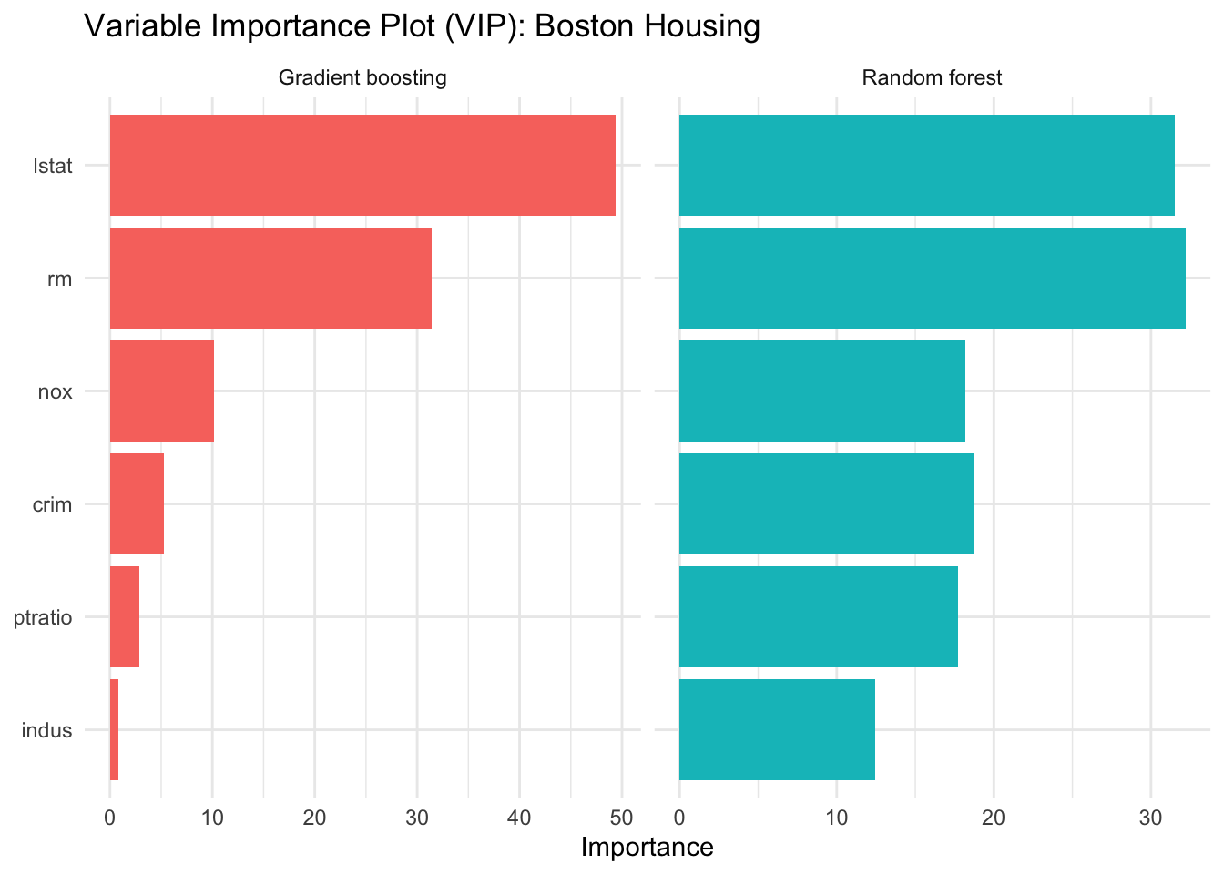
12.8.2 Variable Importance for Pima Diabetes
pima_rf_imp <- importance(pima_rf, type = 1)
pima_rf_imp_df <- data.frame(
    variable = rownames(pima_rf_imp),
    importance = pima_rf_imp[, 1],
    model = "Random forest"
)

pima_gbm_imp <- summary(pima_gbm, n.trees = pima_best, plotit = FALSE)
pima_gbm_imp_df <- data.frame(
    variable = pima_gbm_imp$var,
    importance = pima_gbm_imp$rel.inf,
    model = "Gradient boosting"
)

pima_imp_df <- bind_rows(pima_rf_imp_df, pima_gbm_imp_df)

pima_imp_df |>
    ggplot(aes(x = reorder(variable, importance), y = importance, fill = model)) +
    geom_col(show.legend = FALSE) +
    coord_flip() +
    facet_wrap(~ model, scales = "free_x") +
    labs(
        title = "Variable Importance Plot (VIP): Pima Diabetes",
        x = NULL,
        y = "Importance"
    ) +
    theme_minimal()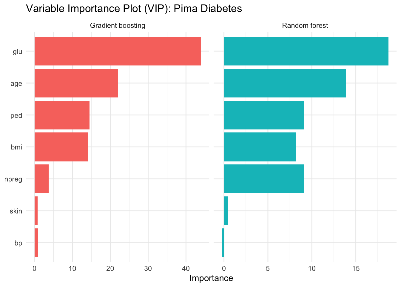
The importance rankings are often more stable than the splits of a single tree. They do not tell us the direction of an effect or the shape of a relationship, but they highlight the predictors that the ensemble relies on most heavily.
12.9 Interpretation and Practical Considerations
Ensembles provide strong performance and stable summaries, but they also come with interpretive costs. In descriptive settings, a few considerations are especially relevant:
- Transparency is reduced compared to a single tree, so summaries like variable importance and partial dependence become essential.
- Hyperparameters influence results, including tree depth, learning rate, and the number of trees. We gain stability but also introduce modeling choices that should be documented.
- Communication can focus on patterns that persist across methods, for example predictors that are consistently ranked high in both random forests and boosting.
These points encourage a balanced stance. Ensembles are not replacements for careful descriptive reasoning, but they can help confirm and stabilize the patterns that single trees suggest.
12.10 Summary and Key Takeaways
- Bagging reduces variance by averaging trees fit to bootstrap samples, with OOB error as a natural diagnostic.
- Random forests add predictor subsampling, which decorrelates trees and often improves stability and accuracy.
- Gradient boosting builds trees sequentially and yields flexible fits, with interpretability depending on extracted summaries.
- Variable importance provides a robust descriptive ranking, but it should be paired with substantive interpretation and complementary plots.
12.11 Looking Ahead
Ensembles shift attention from individual decision rules to stable summaries of model behavior. The next chapter expands this idea by surveying interpretable machine learning approaches that help us understand complex models, including ensembles, through structured diagnostics and explanations.