18Automated Feature Engineering and Interaction Discovery
18.1 Introduction: From Model Search to Feature Space Search
In the previous chapter, we framed AutoML as a descriptive instrument for comparing model families under a common validation protocol. That perspective can be extended in a natural way. Beyond searching over algorithms and hyperparameters, we can also search over representations of the predictors themselves.
Automated feature engineering refers to procedures that generate, screen, and select transformed or combined predictors, often at scale. In tabular settings, this frequently includes nonlinear transformations, pairwise interactions, and simple basis expansions. The goal is not to replace substantive understanding of variables, but to broaden the set of candidate structures that can be evaluated transparently.
This chapter develops that workflow in a reproducible R implementation. We focus on interaction discovery and transformed predictors in a regression setting, then discuss interpretation limits and reporting choices that keep conclusions technically grounded.
18.2 Why Feature Engineering Can Be Automated in Descriptive Work
Earlier in the book, we repeatedly saw that model conclusions depend on how signal is represented. If an important interaction is omitted, an additive model may appear systematically biased in parts of the covariate space. If a relation is nonlinear, raw linear terms can underfit even when model diagnostics look acceptable in aggregate.
A modest automated feature engineering workflow can support descriptive analysis by helping us:
detect candidate nonlinear structure that is not visible in additive baselines,
rank interaction candidates under a common cross validation design,
compare several near-optimal representations instead of one handcrafted specification,
document feature space uncertainty, not only parameter uncertainty.
As in the previous chapter, these are predictive and descriptive statements about fitted behavior under observed data conditions. They do not, by themselves, identify causal effects.
18.3 A Formal View: Search Over Feature Mappings
Let \(X \in \mathbb{R}^{n \times p}\) denote the original predictor matrix and \(y\) the outcome. A feature engineering procedure defines a mapping family
where each mapping can represent, for example, polynomial terms, logarithmic transforms, or interactions. For a chosen modeling algorithm \(\mathcal{A}\) with parameters \(\theta\), we evaluate candidates of the form
with \(\widehat{R}\) estimated by cross validation or a related resampling protocol.
In practice, this search can be large. A key methodological point is that search design (candidate library, screening rule, evaluation budget) is part of the inferential context and should be reported explicitly.
18.4 Running Example: Boston Housing With a Transparent Candidate Library
To remain consistent with the previous chapters, we use the Boston housing data and predict medv. We first fit a baseline additive linear model, then evaluate engineered candidates one at a time on top of that baseline.
We keep a final holdout test set untouched during candidate screening. This separation helps reduce optimism after searching across many engineered terms.
18.5 A Reproducible Evaluation Engine
We implement helper functions for fold assignment and cross validated RMSE. The code below is intentionally compact and explicit, so that each design choice is auditable.
rmse <-function(actual, predicted) {sqrt(mean((actual - predicted)^2))}make_folds <-function(n, k =5, seed =123) {set.seed(seed)sample(rep(seq_len(k), length.out = n))}cv_rmse_lm <-function(data, formula_obj, fold_id) { k <-length(unique(fold_id)) fold_errors <-numeric(k)for (fold inseq_len(k)) { train_fold <- data[fold_id != fold, , drop =FALSE] valid_fold <- data[fold_id == fold, , drop =FALSE] fit <-lm(formula_obj, data = train_fold) pred <-as.numeric(predict(fit, newdata = valid_fold)) fold_errors[fold] <-rmse(valid_fold[[target]], pred) } tibble::tibble(mean_rmse =mean(fold_errors),sd_rmse =sd(fold_errors) )}
18.6 Constructing Candidate Features
For each predictor, we generate two transformation candidates, a quadratic term and a log transformation. We also generate all pairwise interactions among the selected predictors.
This library is not exhaustive, but it is broad enough to illustrate automated screening. In applied projects, candidate generation is often guided by domain constraints, monotonicity expectations, and operational interpretability requirements.
18.7 Screening Candidates by Cross Validated Improvement
We now evaluate each candidate term by augmenting the baseline formula with one additional engineered feature and measuring out of fold RMSE.
The ranking helps us identify promising terms, while the SD column provides context about stability across folds. Small differences should be interpreted cautiously when they are comparable to fold level variability.
18.8 Building an Engineered Model From Top Candidates
A practical compromise between flexibility and readability is to keep only the strongest positive candidates. Here we retain up to five terms with positive estimated gain.
This test set comparison is only one realization, but it indicates whether screened candidates transfer beyond the resampling environment used during selection.
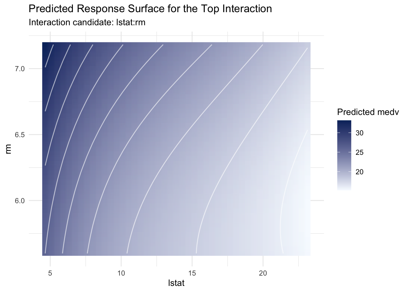
18.9 Inspecting the Interaction Signal
Screening tables are useful, but interaction discovery is often easier to communicate w ith a response surface. We extract the top ranked interaction term, if available, and visualize fitted values while keeping other predictors at their analysis set medians.
if (nrow(top_interaction) ==1) { vars <-strsplit(top_interaction$term[1], ":", fixed =TRUE)[[1]] v1 <- vars[1] v2 <- vars[2] grid_v1 <-seq(as.numeric(quantile(analysis_data[[v1]], 0.1)),as.numeric(quantile(analysis_data[[v1]], 0.9)),length.out =45 ) grid_v2 <-seq(as.numeric(quantile(analysis_data[[v2]], 0.1)),as.numeric(quantile(analysis_data[[v2]], 0.9)),length.out =45 ) surface_data <-expand.grid(x1 = grid_v1,x2 = grid_v2 )names(surface_data) <-c(v1, v2)for (p in predictors) {if (!(p %in%c(v1, v2))) { surface_data[[p]] <-median(analysis_data[[p]]) } } surface_data$pred <-as.numeric(predict(engineered_fit, newdata = surface_data)) surface_data |>ggplot(aes(x = .data[[v1]], y = .data[[v2]], z = pred, fill = pred)) +geom_raster(interpolate =TRUE) +geom_contour(color ="white", alpha =0.6) +scale_fill_gradient(low ="#f7fbff", high ="#08306b") +labs(title ="Predicted Response Surface for the Top Interaction",subtitle =paste("Interaction candidate:", top_interaction$term[1]),x = v1,y = v2,fill ="Predicted medv" ) +theme_minimal()}
The surface should be read as model behavior conditional on fixed values of remaining predictors. It is a useful descriptive map, but not direct evidence of causal interaction.
18.10 Practical Considerations and Failure Modes
Automated feature engineering can increase descriptive resolution, but several risks are worth monitoring.
Search induced optimism can appear when large candidate libraries are screened with weak validation protocols.
Collinearity inflation can destabilize coefficient level interpretation in engineered linear models.
Data leakage can occur if transformations use information outside the analysis fold.
Interpretability drift can arise when many engineered terms are retained without pruning.
These issues do not invalidate automated workflows. They highlight why fold aware preprocessing, explicit holdout testing, and conservative reporting are central parts of the methodology.
18.11 Reporting Guidelines for Automated Feature Engineering
For transparent descriptive reporting, it is often helpful to document:
candidate generation rules (which transforms and interactions were considered),
validation design and random seeds,
selection criterion (for example, improvement in cross validated RMSE),
final retained terms and their practical contribution,
holdout performance relative to a simpler baseline.
When several engineered specifications are near tied, presenting a small candidate set can be more informative than emphasizing a single winner.
18.12 Summary and Key Takeaways
Automated feature engineering extends AutoML logic from model space to feature space.
Interaction and transformation screening can reveal predictive structure not captured by additive baselines.
Cross validated ranking is most useful when read together with variability measures and holdout confirmation.
Interaction surfaces support interpretation, while remaining conditional predictive summaries.
Transparent documentation of the candidate library and validation design is essential for credible descriptive conclusions.
18.13 Looking Ahead
This chapter focused on representation search in a controlled tabular workflow. In the next chapters, we turn to integrated case studies where model search, feature engineering, and interpretation are combined in full descriptive analyses for policy, health, and business contexts.