11Classification Trees and Confusion Matrix Insights
11.1 Introduction: From Segments to Classes
Regression trees helped us segment continuous outcomes into interpretable subgroups. Classification trees extend the same recursive partitioning logic to categorical outcomes, where each leaf predicts a class label rather than a mean value. The descriptive appeal is similar, a small set of decision rules can summarize how predictors separate categories.
In this chapter we focus on how classification trees communicate structure and performance. We emphasize confusion matrices (including their binary 2×2 form), class probabilities and the Brier score, and the interpretive meaning of splits, rather than only predictive accuracy.
11.2 The Classification Tree Idea
Classification trees divide the predictor space into regions that are as class homogeneous as possible. Each split is chosen to reduce impurity in the child nodes. Common impurity measures include the Gini index and cross-entropy (deviance). For the Gini index (Breiman et al. 2017),
\[
G = 1 - \sum_{k=1}^K p_k^2,
\]
where \(p_k\) is the proportion of class \(k\) in a node. A good split reduces impurity by creating child nodes with more concentrated class distributions.
As with regression trees, classification trees are piecewise constant models. They are not smooth, but they are interpretable, a valuable feature when the goal is explanation and communication.
11.3 A Reproducible Example with the Iris Data
We use the classic iris dataset. The response is species, and the predictors are the four flower measurements. The dataset is small enough to examine directly, and it produces a compact tree.
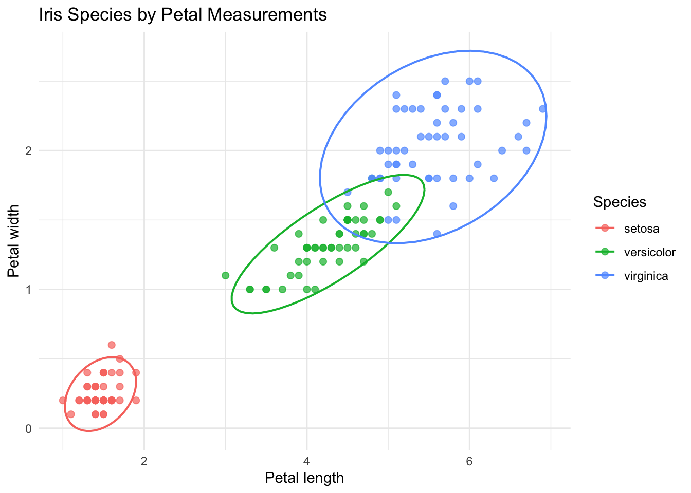
Before fitting a tree, we can visualize how two features separate the classes. This is not required, but it provides intuition for the splits that follow.
iris |>ggplot(aes(x = Petal.Length, y = Petal.Width, color = Species)) +geom_point(alpha =0.7, size =2) +stat_ellipse(type ="norm", linewidth =0.7) +labs(title ="Iris Species by Petal Measurements",x ="Petal length",y ="Petal width" ) +theme_minimal()
11.4 Fitting a Classification Tree
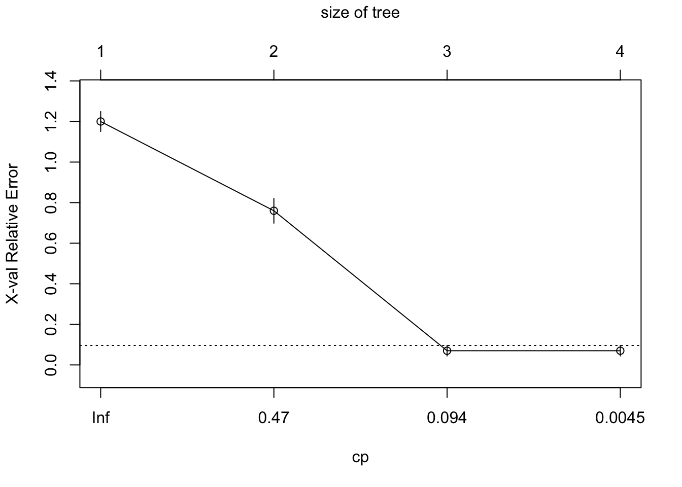
We fit a tree using rpart with method = "class". We set a small complexity parameter to grow an initial tree and then prune it based on cross-validated error.
set.seed(123)class_tree <-rpart( Species ~ ., data = iris,method ="class",control =rpart.control(minsplit =10, cp =0.001))
As in the regression case, the console output is not the most readable summary. We move quickly to pruning diagnostics and visual representations.
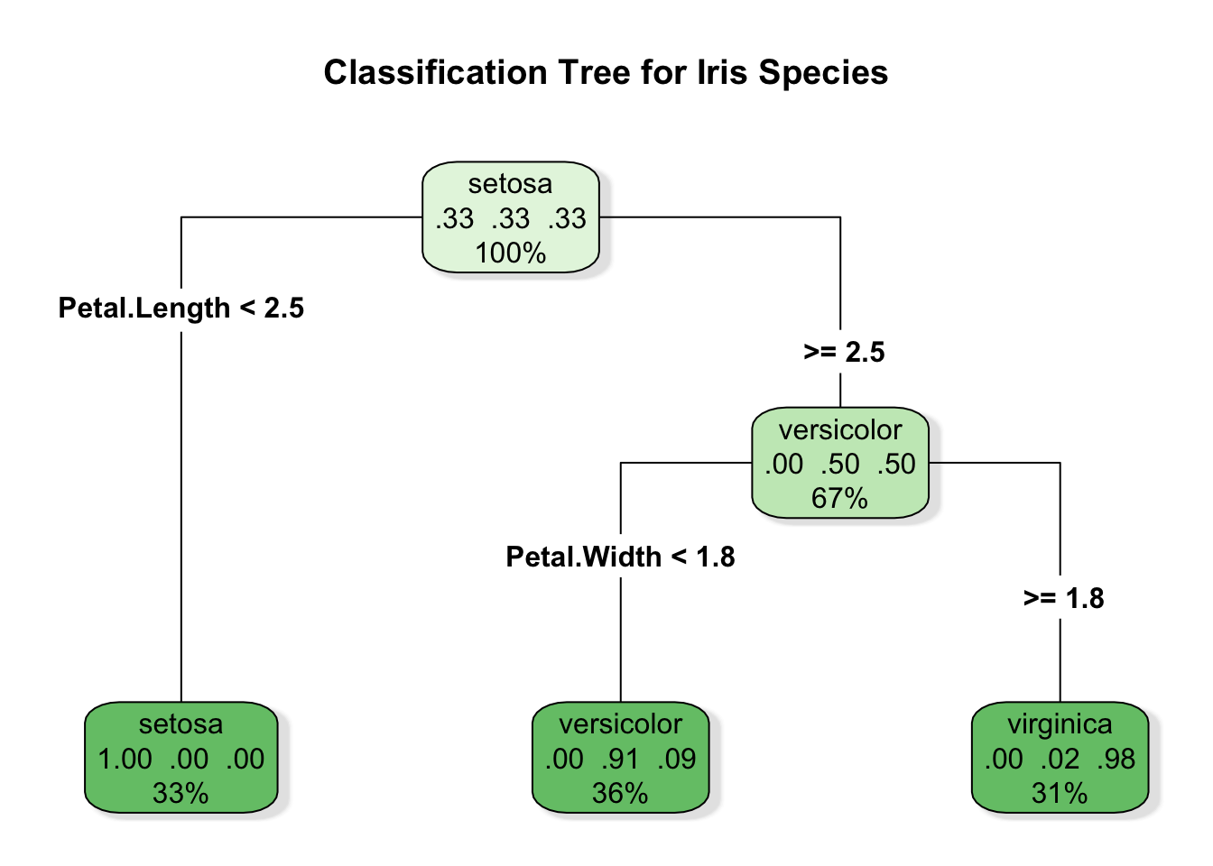
The plot below emphasizes readability, with class labels and node sizes that make the main splits easy to follow.
rpart.plot( pruned_class_tree,type =4,extra =104,fallen.leaves =TRUE,box.palette ="Greens",branch.lty =1,shadow.col ="gray90",main ="Classification Tree for Iris Species")
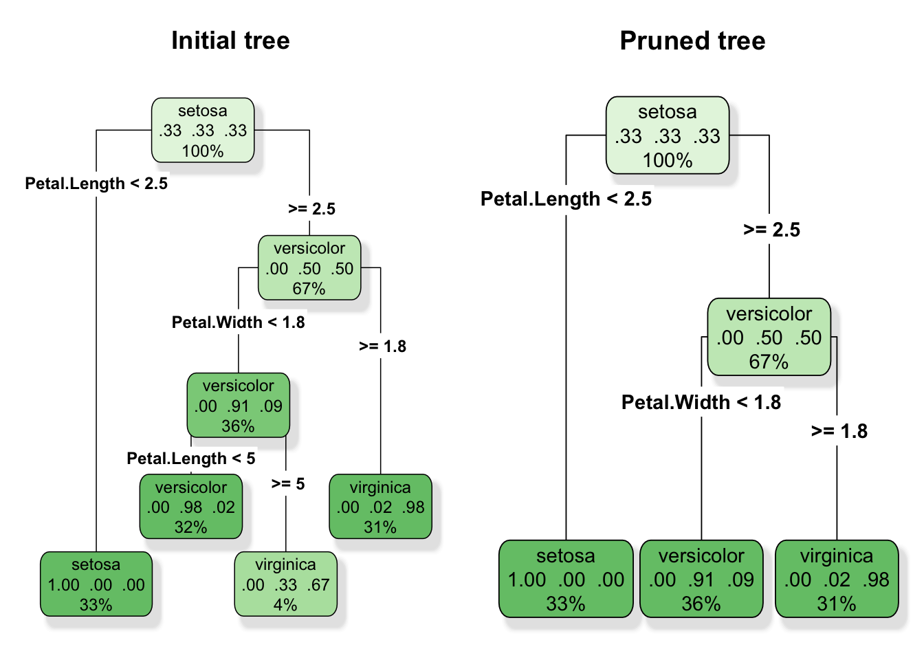
To see the effect of pruning more directly, we can compare the initial tree to the pruned tree side by side. The pruned version is smaller, with fewer terminal nodes and clearer rules.
Classification trees are often evaluated with a confusion matrix. Even in descriptive work, the matrix reveals where the tree distinguishes classes well and where it confuses them.
pred_class <-predict(pruned_class_tree, iris, type ="class")conf_mat <-table(Actual = iris$Species, Predicted = pred_class)conf_mat_df <-as.data.frame.matrix(conf_mat)conf_mat_df <- tibble::rownames_to_column(conf_mat_df, var ="Actual")conf_mat_df |>gt(rowname_col ="Actual")
setosa
versicolor
virginica
setosa
50
0
0
versicolor
0
49
1
virginica
0
5
45
We can also compute summary metrics. For a multiclass setting, it is common to report overall accuracy and macro-averaged precision, recall, and F1 scores.
The confusion matrix gives a granular view of errors, while the macro averages summarize performance across classes. In descriptive contexts, these summaries indicate whether the tree is separating groups in a meaningful way, rather than merely fitting noise.
11.6.1 The 2×2 Case: Binary Classification
The iris example uses three classes, but in practice the most common setting is a binary outcome: two classes such as Yes/No, positive/negative, or event/no-event. The confusion matrix then takes a specific 2×2 form that has its own conventional vocabulary worth knowing, because it appears throughout the later chapters.
The four cells of a binary confusion matrix are:
Predicted Negative
Predicted Positive
Actual Negative
True Negative (TN)
False Positive (FP)
Actual Positive
False Negative (FN)
True Positive (TP)
From these four counts, the summary metrics we computed above reduce to familiar binary formulas:
Precision: \(TP / (TP + FP)\) — of those predicted positive, how many actually are
Recall (also called sensitivity): \(TP / (TP + FN)\) — of those actually positive, how many were caught
Specificity: \(TN / (TN + FP)\) — of those actually negative, how many were correctly identified as such
In descriptive work, the confusion matrix is most useful not as a performance scorecard but as a diagnostic: it shows whether a tree is systematically confusing one class for another, which can reveal structure in the data. A tree that consistently misclassifies one group is telling you something about how those cases are distributed in the predictor space, not just about model quality.
The layout of the matrix (which class is “positive”) matters for interpretation. When one class carries more practical weight (for instance, disease cases in a health setting, or high-value customers in a business setting), it is conventional to treat it as the positive class so that false negatives and false positives have a clear asymmetric meaning.
11.6.2 The Brier Score: Evaluating Predicted Probabilities
The metrics above, that is, accuracy, precision, recall, and F1, all evaluate hard class predictions: the tree assigns each observation to a single class and we check whether it was right. But classification trees also produce class probabilities at each leaf (the proportion of training observations of each class in that node), and those probabilities carry information that hard labels discard.
The Brier score measures how well-calibrated predicted probabilities are, by computing the average squared deviation between the predicted probability and the actual binary outcome (BRIER 1950):
where \(p_i\) is the predicted probability of the positive class for observation \(i\), and \(y_i\) is 1 if the event occurred and 0 otherwise. A Brier score of 0 means perfect probability predictions; a score of 1 is the worst possible. A naive model that always predicts the base rate has a Brier score equal to \(p(1-p)\), which provides a useful reference point.
In a binary setting, the computation is straightforward:
# Brier score for a binary outcome (illustration with a two-class version of iris)iris_binary <- iris |>filter(Species !="virginica") |>mutate(Species =droplevels(Species))tree_binary <-rpart( Species ~ .,data = iris_binary,method ="class",control =rpart.control(cp =0.001))pred_prob_binary <-predict(tree_binary, iris_binary, type ="prob")[, "versicolor"]actual_binary <-as.integer(iris_binary$Species =="versicolor")brier_score <-mean((pred_prob_binary - actual_binary)^2)brier_score
[1] 0
The Brier score is most informative when compared to this baseline:
A Brier score well below the baseline suggests the model’s probability estimates are adding genuine information beyond the marginal class distribution. In descriptive work, this matters because it indicates whether the leaf-level probability estimates are trustworthy enough to support interpretation, for instance, when communicating risk gradients or ranking observations by predicted likelihood.
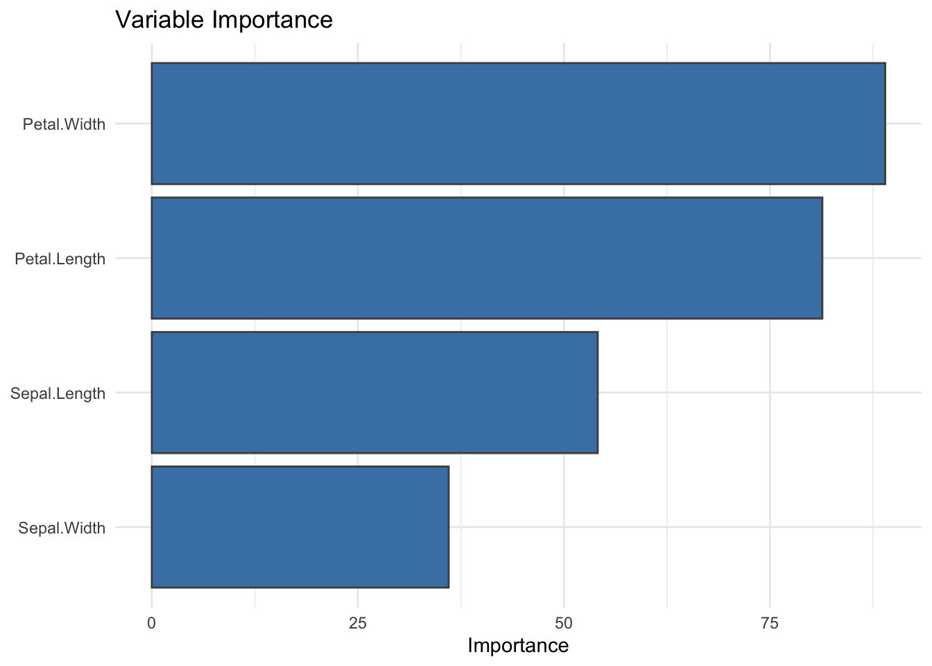
11.7 Variable Importance for Classification Trees
Trees provide a built-in measure of variable importance, based on how much each variable reduces impurity across splits. This is a useful complement to the tree structure itself.
Importance is best read as a ranking. It suggests which predictors shape the tree most strongly, while the split rules clarify how those predictors partition the classes.
11.8 Interpretation and Practical Considerations
Classification trees are attractive because they express decision boundaries as explicit rules. That said, the following considerations are often important in practice:
Class probabilities can be more informative than hard labels, especially when classes overlap.
Imbalanced classes may require cost-sensitive splits or reweighting to avoid dominance by the majority class.
Stability remains a concern, small changes in data can alter splits, so we treat a single tree as a descriptive summary rather than a definitive model.
These points reinforce the value of using trees as one component in a broader descriptive toolkit.
11.9 Summary and Key Takeaways
Classification trees extend recursive partitioning to categorical outcomes, yielding interpretable decision rules.
Pruning is essential for readability and stability, and cross-validation offers a reasonable default for tree size.
Confusion matrices reveal where the tree succeeds or confuses classes, while macro metrics summarize overall balance.
In binary classification, the 2×2 confusion matrix introduces a standard vocabulary (true positives, false negatives, specificity) that supports asymmetric interpretation when one class carries more practical weight.
The Brier score complements hard-label metrics by evaluating the quality of predicted probabilities, using the base rate as a natural reference point.
Variable importance provides a ranking of predictors, best interpreted alongside the actual split structure.
11.10 Looking Ahead
Classification trees provide a transparent baseline, but they can be unstable and sometimes less accurate than ensemble methods. The next chapter introduces tree ensembles, where many trees are combined to improve stability and performance while retaining interpretive cues.
Breiman, Leo, Jerome H. Friedman, Richard A. Olshen, and Charles J. Stone. 2017. Classification and Regression Trees. Routledge. https://doi.org/10.1201/9781315139470.