| Interpretive question | Scope | Typical tools | Method class |
|---|---|---|---|
| Which variables matter most overall? | Global | Permutation importance, impurity based importance | Mostly model agnostic |
| How does the response vary with one predictor? | Global | Partial dependence, accumulated local effects | Mostly model agnostic |
| Why this specific prediction? | Local | Local perturbation profiles, Shapley style attributions | Model agnostic or model specific |
| Can we summarize a black box with simple rules? | Global | Surrogate trees, sparse rule lists | Post hoc |
13 Interpretable ML: An Overview
13.1 Introduction: From Predictive Strength to Explanatory Clarity
In the previous chapters we used tree based models, including ensembles, as descriptive instruments. We saw that ensembling can improve stability and predictive performance, but we also saw a recurrent tension, as model complexity grows, direct inspection becomes harder.
Interpretable machine learning addresses this tension. The goal is not to choose between prediction and interpretation in absolute terms. Instead, we try to recover useful explanations about model behavior, and to do so in a way that is technically sound and substantively meaningful.
This chapter provides a conceptual map of interpretable ML. We distinguish global and local explanations, model specific and model agnostic methods, and intrinsic and post hoc interpretability. We then work through a reproducible example that illustrates how these ideas can be used in practice.
13.2 What We Mean by “Interpretability”
Interpretability is often used loosely, so it helps to be explicit. In this book, we treat an explanation as useful when it helps us answer at least one of the following questions:
- Which predictors are most associated with the model output?
- How does the predicted response change when a predictor changes, while others are held fixed or averaged over?
- Why did the model produce a particular prediction for one observation?
These questions are related, but not identical. Variable ranking gives a broad sense of relevance, functional summaries describe shape, and case level explanations address specific predictions. A single summary rarely answers all three questions.
Interpretability is also contextual. An explanation that is useful for exploratory analysis may not be sufficient for auditing, policy communication, or scientific reporting. For that reason, we usually combine several complementary summaries.
13.3 A Practical Taxonomy of Interpretability Methods
Two dimensions are especially useful in practice:
- Scope: global methods summarize model behavior over many observations, whereas local methods focus on one prediction or a small neighborhood.
- Model dependence: model specific methods use internal model structure, whereas model agnostic methods only require predictions.
The distinction between intrinsic and post hoc interpretability is also useful. Intrinsic interpretability is built into the model class (for example, a small decision tree). Post hoc interpretability is added after fitting a flexible model.
This taxonomy is not rigid. Many methods can be adapted to different settings. It still provides a useful framework for deciding what to compute and how to communicate it.
13.4 Running Example: Random Forest on Boston Housing Data
To make the ideas concrete, we use the Boston housing dataset and fit a random forest model for medv (median home value). The model is intentionally moderate in complexity, which keeps interpretation manageable while preserving nonlinear structure.
data(Boston, package = "MASS")

set.seed(123)
idx <- sample(seq_len(nrow(Boston)), size = 0.7 * nrow(Boston))
train <- Boston[idx, ]
test <- Boston[-idx, ]

predictors <- c("lstat", "rm", "ptratio", "indus", "nox", "crim")
rf_formula <- as.formula(paste("medv ~", paste(predictors, collapse = " + ")))

set.seed(123)
rf_fit <- randomForest(
    rf_formula,
    data = train,
    ntree = 500,
    mtry = 2,
    importance = TRUE
)

rf_pred <- predict(rf_fit, newdata = test)
rf_rmse <- sqrt(mean((test$medv - rf_pred)^2))

rf_rmse
[1] 3.5575The test RMSE gives a baseline for predictive quality. Interpretability summaries should be read alongside this baseline, because explanations of a weak model are often unstable or misleading.
13.5 Global Explanation 1: Permutation Importance
Permutation importance measures how much model error increases when a predictor is randomly shuffled. Shuffling breaks the predictor response relationship while preserving the predictor’s marginal distribution.
If shuffling variable \(X_j\) increases error substantially, the model appears to rely on \(X_j\) for prediction. Formally, for an error function \(L\) (Breiman 2001; Fisher, Rudin, and Dominici 2019),
\[ I_j = \mathbb{E}\left[L\left(Y, \hat{f}(X_{-j}, \pi(X_j))\right)\right] - \mathbb{E}\left[L\left(Y, \hat{f}(X)\right)\right], \]
where \(\pi(X_j)\) denotes a random permutation of feature \(j\).
In the next chapter, we return to permutation importance with an explicit finite sample estimator, so the conceptual definition introduced here is connected directly to implementation and reporting practice.
We now implement this procedure for our random forest model. We define a function that computes permutation importance for each predictor by repeatedly shuffling it and recording the change in test RMSE. We then apply this function to all six predictors and visualize the results to identify which features the model relies on most heavily.
perm_importance <- function(model, data, outcome, vars, n_repeats = 8, seed = 123) {
    set.seed(seed)
    base_pred <- predict(model, newdata = data)
    base_rmse <- sqrt(mean((data[[outcome]] - base_pred)^2))

    results <- lapply(vars, function(v) {
        deltas <- numeric(n_repeats)
        for (b in seq_len(n_repeats)) {
            perm_data <- data
            perm_data[[v]] <- sample(perm_data[[v]])
            perm_pred <- predict(model, newdata = perm_data)
            perm_rmse <- sqrt(mean((data[[outcome]] - perm_pred)^2))
            deltas[b] <- perm_rmse - base_rmse
        }
        tibble::tibble(
            variable = v,
            mean_delta_rmse = mean(deltas),
            sd_delta_rmse = sd(deltas)
        )
    })

    dplyr::bind_rows(results) |>
        arrange(desc(mean_delta_rmse))
}

perm_imp <- perm_importance(
    model = rf_fit,
    data = test,
    outcome = "medv",
    vars = predictors,
    n_repeats = 10
)

perm_imp |>
    gt() |>
fmt_number(columns = where(is.numeric), decimals = 3)| variable | mean_delta_rmse | sd_delta_rmse |
|---|---|---|
| lstat | 3.831 | 0.319 |
| rm | 3.026 | 0.305 |
| nox | 0.446 | 0.057 |
| ptratio | 0.399 | 0.113 |
| crim | 0.158 | 0.076 |
| indus | 0.146 | 0.033 |
perm_imp |>
    ggplot(aes(x = reorder(variable, mean_delta_rmse), y = mean_delta_rmse)) +
    geom_col(fill = "steelblue", alpha = 0.85) +
    geom_errorbar(
        aes(ymin = mean_delta_rmse - sd_delta_rmse, ymax = mean_delta_rmse + sd_delta_rmse),
        width = 0.15,
        color = "gray25"
    ) +
    coord_flip() +
    labs(
        title = "Permutation Importance for the Random Forest",
        subtitle = "Error bars show ±1 standard deviation across repeated shuffles",
        x = NULL,
        y = "Increase in RMSE after permutation"
    ) +
    theme_minimal()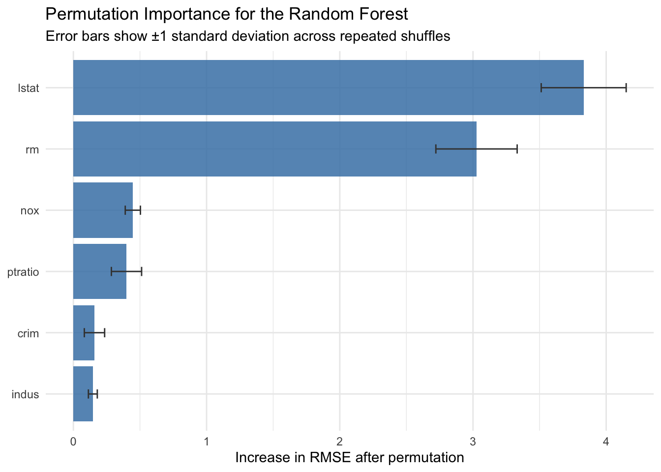
Permutation importance is often more comparable across model classes than impurity based scores. At the same time, it can be sensitive to correlated predictors, because one predictor can partially substitute for another.
13.6 Global Explanation 2: Partial Dependence
A partial dependence profile averages model predictions over the observed distribution of other features, while varying one focal predictor. For predictor \(X_s\) (Friedman 2001),
\[ \hat{f}_{PD}(x_s) = \frac{1}{n}\sum_{i=1}^{n} \hat{f}(x_s, x_{i,C}), \]
where \(C\) indexes all non focal predictors.
To illustrate this, we compute the partial dependence profile for lstat (percentage of lower status population). We create a grid of lstat values spanning the 5th to 95th percentile, then for each grid point we set all observations to that lstat value and average the model predictions. The resulting curve shows how the expected prediction changes as lstat varies.
partial_dependence <- function(model, data, variable, grid_values) {
    pd_values <- sapply(grid_values, function(g) {
        new_data <- data
        new_data[[variable]] <- g
        mean(predict(model, newdata = new_data))
    })

    tibble::tibble(
        value = grid_values,
        pd = pd_values,
        variable = variable
    )
}

lstat_grid <- seq(
    from = quantile(train$lstat, 0.05),
    to = quantile(train$lstat, 0.95),
    length.out = 40
)

pd_lstat <- partial_dependence(
    model = rf_fit,
    data = train,
    variable = "lstat",
    grid_values = lstat_grid
)

pd_lstat |>
    ggplot(aes(x = value, y = pd)) +
    geom_line(color = "darkred", linewidth = 1) +
    labs(
        title = "Partial Dependence of medv on lstat",
        x = "lstat",
        y = "Average predicted medv"
    ) +
    theme_minimal()
This curve describes model behavior, not a causal response curve. It is best interpreted as a summary of how predictions tend to vary with lstat within the observed data region.
13.7 Local Explanation: A Case Based Perturbation Profile
Global summaries can hide heterogeneity. Local explanations focus on one observation and ask how its prediction changes when selected features are perturbed.
For this demonstration, we select a single observation from the test set and examine how its prediction would change if we replaced each of its feature values with low (10th percentile) or high (90th percentile) values from the training distribution. This counterfactual approach reveals which features have the largest leverage on this particular prediction.
case_id <- 10
case_obs <- test[case_id, , drop = FALSE]
case_pred <- as.numeric(predict(rf_fit, newdata = case_obs))

local_profile <- lapply(predictors, function(v) {
    q_low <- as.numeric(quantile(train[[v]], 0.10))
    q_high <- as.numeric(quantile(train[[v]], 0.90))

    case_low <- case_obs
    case_high <- case_obs
    case_low[[v]] <- q_low
    case_high[[v]] <- q_high

    pred_low <- as.numeric(predict(rf_fit, newdata = case_low))
    pred_high <- as.numeric(predict(rf_fit, newdata = case_high))

    tibble::tibble(
        variable = v,
        prediction_low = pred_low,
        prediction_high = pred_high,
        delta_low = pred_low - case_pred,
        delta_high = pred_high - case_pred
    )
}) |>
    dplyr::bind_rows()

local_profile |>
    transmute(
        Variable = variable,
        `Prediction (10th pct)` = prediction_low,
        `Prediction (90th pct)` = prediction_high,
        `Change from observed prediction, 10th pct` = delta_low,
        `Change from observed prediction, 90th pct` = delta_high
    ) |>
    gt() |>
fmt_number(columns = where(is.numeric), decimals = 2)| Variable | Prediction (10th pct) | Prediction (90th pct) | Change from observed prediction, 10th pct | Change from observed prediction, 90th pct |
|---|---|---|---|---|
| lstat | 22.54 | 13.98 | 4.29 | −4.26 |
| rm | 18.37 | 24.54 | 0.12 | 6.29 |
| ptratio | 20.13 | 18.66 | 1.88 | 0.41 |
| indus | 19.74 | 18.93 | 1.49 | 0.68 |
| nox | 18.81 | 18.86 | 0.57 | 0.62 |
| crim | 18.39 | 19.52 | 0.15 | 1.27 |
This local profile is a sensitivity summary, not an additive attribution. It is still useful in descriptive work because it shows which feature perturbations move this specific prediction the most.
13.8 Interpretable Surrogates: Approximating a Complex Model with a Tree
Another common strategy is to fit an interpretable surrogate model to predictions from a complex model. Here we fit a shallow regression tree to random forest predictions.
rf_train_pred <- predict(rf_fit, newdata = train)

surrogate_tree <- rpart(
    rf_train_pred ~ lstat + rm + ptratio + indus + nox + crim,
    data = train,
    method = "anova",
    control = rpart.control(maxdepth = 3, minsplit = 40, cp = 0.001)
)

rpart.plot(
    surrogate_tree,
    type = 2,
    extra = 101,
    fallen.leaves = TRUE,
    box.palette = "Blues",
    main = "Surrogate Tree for Random Forest Predictions"
)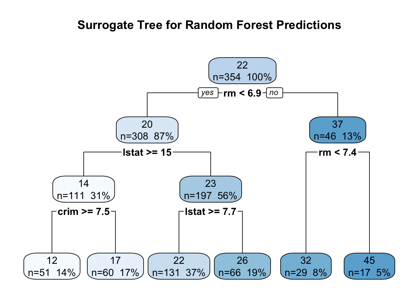
To assess how well this surrogate captures the original model’s behavior, we compute fidelity diagnostics on the test set. We generate predictions from both the random forest and the surrogate tree, then calculate the correlation between them and the RMSE of their differences. High correlation and low RMSE indicate that the simpler tree approximates the complex model reasonably well within the observed data region.
rf_test_pred <- predict(rf_fit, newdata = test)
sur_test_pred <- predict(surrogate_tree, newdata = test)

surrogate_fidelity_cor <- cor(rf_test_pred, sur_test_pred)
surrogate_fidelity_rmse <- sqrt(mean((rf_test_pred - sur_test_pred)^2))

tibble::tibble(
    Metric = c("Correlation with RF predictions", "RMSE against RF predictions"),
    Value = c(surrogate_fidelity_cor, surrogate_fidelity_rmse)
) |>
    gt() |>
fmt_number(columns = Value, decimals = 3)| Metric | Value |
|---|---|
| Correlation with RF predictions | 0.939 |
| RMSE against RF predictions | 3.107 |
Surrogate models can make complex behavior easier to communicate, but they remain approximations. Fidelity diagnostics help us avoid treating the surrogate as if it were the original model.
13.9 Interpretation Pitfalls and Good Practice
Interpretable ML methods are informative, but they are not neutral or assumption free. Several points are worth keeping in view:
- Association is not causation. Explanations describe model behavior under the observed data generating process.
- Correlated predictors complicate attribution. Importance and effect summaries can shift when predictors carry overlapping information.
- Extrapolation risk matters for profile based methods. Curves are most reliable where data support is adequate.
- Stability should be checked. Explanations may vary across resamples, especially in small datasets.
In practice, we often obtain stronger descriptive insight by triangulating, for example, using importance rankings, functional profiles, and local perturbation summaries together.
13.10 Summary and Key Takeaways
This chapter introduced the conceptual foundations of interpretable machine learning and demonstrated a practical workflow for explaining model behavior. Several themes are worth emphasizing:
- Interpretability is multifaceted. Global explanations summarize overall model behavior, while local explanations address individual predictions. Model agnostic methods work across different model classes, while model specific methods exploit internal structure. Both perspectives are valuable.
- Different questions require different tools. Variable importance rankings answer “which features matter?”, partial dependence profiles show “how do predictions vary with a feature?”, and case based perturbations explain “why this specific prediction?”. A single summary rarely answers all relevant questions.
- Explanations are descriptive, not causal. Permutation importance, partial dependence, and other methods describe model behavior under the observed data distribution. They do not identify causal effects or guarantee generalization beyond the training context.
- Context shapes interpretation. An explanation sufficient for exploratory analysis may not meet requirements for auditing, regulatory compliance, or scientific reporting. Always consider the intended use when selecting and presenting interpretability summaries.
- Triangulation strengthens insight. Combining importance rankings, functional profiles, and local explanations helps us build a more complete picture of how a model organizes information. Correlated predictors, nonlinear interactions, and data sparsity all complicate interpretation, so multiple perspectives are often more reliable than a single metric.
The practical examples in this chapter used a random forest on the Boston housing data, but the principles extend naturally to other model classes and application domains.
13.11 Looking Ahead
The following chapters develop each interpretability component in greater technical depth. We begin with feature importance measures, exploring both model specific and model agnostic approaches. We then examine partial dependence and related profile methods that characterize functional relationships. Finally, we introduce Shapley based decompositions, which provide a principled framework for attributing predictions to individual features. Together, these tools offer a more complete descriptive account of how complex models organize information in tabular data.