4Unified Association Measures for Mixed-Type Variables
4.1 Introduction: The Challenge of Mixed-Type Data
Real-world datasets rarely consist of purely continuous or purely categorical variables. A typical health survey contains continuous biomarkers, ordinal symptom scales, categorical diagnoses, and binary treatment indicators. A business database combines numeric sales figures, categorical product types, ordinal customer satisfaction ratings, and binary contract status.
A helpful framing question is: How do we measure association across such mixed data in a unified, comparable way?
Chapter 2 established that different variable types require different association measures. But practitioners often face a practical problem: given a dataset with mixed types, how do we compute a single association matrix that allows us to rank relationships, identify anomalies, and prepare for network analysis or further modeling?
This chapter presents a practical framework for unified association measurement. We aim to:
Survey classical type-specific measures and their limitations
Introduce modern alternatives that are more flexible and often more robust
Build a type-aware framework for selecting appropriate measures
Demonstrate implementation on real mixed-type data
4.2 Variable Type Classification
Association is not a single concept. The way we measure relationships depends on the measurement scale of the variables involved. A correlation coefficient makes sense for two continuous variables, but it becomes misleading when applied to categorical or ordinal data. A good descriptive workflow usually begins by classifying variable types and selecting association measures accordingly.
We classify variables into five types:
Type
Examples
Characteristics
Continuous
income, height, temperature
Interval/ratio scale, numeric measurements
Discrete
count data, number of events
Non-negative integers, often right-skewed
Ordinal
education level, Likert scales
Ordered categories, rank structure matters
Categorical
region, industry, color
Unordered labels, no inherent order
Binary
yes/no, 0/1, presence/absence
Two categories, often treatment or outcome indicator
The core goal is comparability: use measures that help us rank associations across mixed types without forcing invalid assumptions.
4.3 Classical Measures by Variable Type
Classical association measures are well-understood, computationally efficient, and interpretable. However, each is designed for specific type combinations. We review the most important measures organized by the types of variables they handle.
4.3.1 Continuous-Continuous: Pearson and Spearman
Pearson’s\(r\) measures linear association between two continuous variables (Pearson 1895; Anderson 1985). It is scale-invariant, interpretable, and widely understood. However, it has significant limitations:
Sensitive to outliers
Assumes bivariate normality for inference (though we focus on description)
Misses nonlinear relationships (two variables can be perfectly dependent with \(r = 0\))
Spearman’s\(\rho\) ranks data first, then computes Pearson’s \(r\) on ranks (Spearman 1961). This makes it:
Robust to outliers
Sensitive to monotonic (not just linear) relationships
Suitable for ordinal data
# Compare Pearson and Spearman on data with nonlinear associationset.seed(42)data_nonlin <-tibble(x =seq(0, 4, length.out =100),y = x^2+rnorm(100, 0, 2))tibble(Measure =c("Pearson", "Spearman"),r =c(cor(data_nonlin$x, data_nonlin$y, method ="pearson"),cor(data_nonlin$x, data_nonlin$y, method ="spearman") )) |>gt() |>fmt_number(columns = r, decimals =3)
Measure
r
Pearson
0.880
Spearman
0.877
Recommendation: Spearman is often a sensible default for continuous–continuous pairs due to its robustness; Pearson can be helpful when linearity is established and outliers are minimal.
4.3.2 Categorical-Categorical: Cramér’s V
For two categorical variables, Cramér’s V normalizes the chi-square statistic to \([0, 1]\)(David and Cramer 1947):
\[V = \sqrt{\frac{\chi^2}{n(k-1)}}\]
where \(k = \min(\text{rows}, \text{columns})\). This is intuitive and widely used, though it tends to underestimate association in sparse tables.
# Cramér's V for categorical variablescramers_v <-function(x, y) { tab <-table(x, y) chi2 <-suppressWarnings(chisq.test(tab, correct =FALSE)$statistic) n <-sum(tab) k <-min(nrow(tab), ncol(tab))sqrt(as.numeric(chi2) / (n * (k -1)))}# Example: cylinder type vs transmission typemtcars |>summarise(V =cramers_v(factor(cyl), factor(am))) |>gt() |>fmt_number(columns = V, decimals =3)
V
0.523
4.3.3 Continuous-Categorical: Eta-Squared
When a continuous variable varies across groups defined by a categorical variable, eta-squared (\(\eta^2\)) captures the proportion of variance explained (Fisher 1990; Cohen 2013):
Ordinal variables carry rank information that is often best retained. Kendall’s\(\tau\) is a natural choice for ordinal–ordinal associations and is robust to ties (Kendall 1938). Spearman’s\(\rho\) can also be used for ordinal data.
# Ordinal example using a cut of mpgmtcars |>mutate(mpg_ordinal =cut(mpg, breaks =4, ordered_result =TRUE)) |>summarise(spearman =cor(as.numeric(mpg_ordinal), wt, method ="spearman"),kendall =cor(as.numeric(mpg_ordinal), wt, method ="kendall") ) |>gt() |>fmt_number(columns =c(spearman, kendall), decimals =3)
spearman
kendall
−0.777
−0.656
4.3.5 Binary-Binary: Phi Coefficient
Binary variables can be treated as a special case of categorical data. For two binary indicators, the phi coefficient is equivalent to Pearson correlation on 0/1 coding.
# Phi coefficient for two binary variablesphi <-function(x, y) {cor(as.integer(x), as.integer(y))}mtcars |>mutate(am_bin = am ==1, vs_bin = vs ==1) |>summarise(phi =phi(am_bin, vs_bin)) |>gt() |>fmt_number(columns = phi, decimals =3)
phi
0.168
4.4 Modern Alternatives: Beyond Classical Measures
Classical measures work well within their designed domains but lack flexibility. We present modern association measures that offer broader applicability and often improved robustness.
Works for any dimension (univariate, multivariate)
Detects both linear and nonlinear associations
Equals zero if and only if the variables are independent
Is not sensitive to outliers in the same way as Pearson’s \(r\)
The distance correlation is computed from distance matrices of the two variables by centering these matrices and computing their correlation.
# Distance correlation via the energy packagelibrary(energy)# Example mtcars |>summarise(dcor =dcor(mpg, wt),pearson =cor(mpg, wt, method ="pearson") ) |>gt() |>fmt_number(columns =c(dcor, pearson), decimals =3)
dcor
pearson
0.871
−0.868
Practical advantages:
Captures nonlinear relationships
Robust to outliers
Theoretically appealing (zero iff independent)
Disadvantages:
Computationally expensive for large samples
Less interpretable than Pearson’s \(r\) or Spearman’s \(\rho\)
4.4.2 Maximal Information Coefficient (MIC)
The Maximal Information Coefficient(Reshef et al. 2011) measures association by finding the grid partition of the data that maximizes mutual information. It detects diverse functional relationships (linear, nonlinear, exponential, etc.) and is normalized to \([0, 1]\).
Strengths:
Detects diverse functional relationships
Symmetric and normalized
No assumption about relationship shape
Weaknesses:
Computationally demanding
Can be noisy with small sample sizes
Requires specialized software
# MIC example (requires the minerva package)library(minerva)# Compute MIC for a pairset.seed(42) x <-rnorm(200) y <- x^2+rnorm(200, 0, 0.5) mic_result <-mine(x, y)tibble(Measure ="MIC",Value = mic_result$MIC ) |>gt() |>fmt_number(columns = Value, decimals =3)
Measure
Value
MIC
0.729
4.4.3 Mutual Information
Mutual information (MI) quantifies the amount of information one variable contains about another (Shannon 1948; Cover and Thomas 2001):
Interpretation challenge: MI is measured in “nats” or “bits” and lacks an intuitive 0-1 scale, making comparisons across variable pairs difficult without normalization.
Copulas separate marginal distributions from the dependence structure (Sklar 1959). Common copula-derived measures include Kendall’s tau and Spearman’s rho, which are rank-based and capture dependence structure independent of marginal scales.
Given the diversity of measures, we need a practical approach that applies the most appropriate measure to each variable pair based on their types.
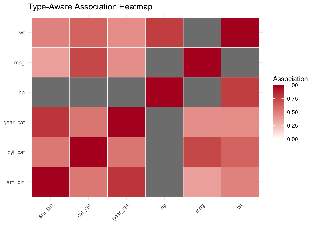
4.5.1 Association Measure Selection Matrix
The table below summarizes recommended measures for each type combination. This consolidated matrix serves as the primary reference for selecting appropriate measures:
X → Y
Continuous
Discrete
Ordinal
Categorical
Binary
Continuous
Spearman (default), Pearson, distance correlation
Spearman, distance correlation
Spearman, polyserial
\(\eta^2\), distance correlation
Point-biserial, \(\eta^2\)
Discrete
Spearman, distance correlation
Spearman
Spearman
\(\eta^2\), distance correlation
\(\eta^2\)
Ordinal
Spearman, polyserial
Spearman
Kendall’s \(\tau\), Spearman
Polychoric, Cramér’s V
Rank-biserial
Categorical
\(\eta^2\), distance correlation
\(\eta^2\), distance correlation
Polychoric, Cramér’s V
Cramér’s V, mutual information
\(\phi\), Cramér’s V
Binary
Point-biserial, \(\eta^2\)
\(\eta^2\)
Rank-biserial
\(\phi\), Cramér’s V
\(\phi\)
Rationale for selections:
Continuous-Continuous: Use Spearman as default (robust to outliers); add distance correlation to detect nonlinearity
Continuous-Categorical: Use \(\eta^2\) to measure variance explained by group membership
Categorical-Categorical: Use Cramér’s V (normalized chi-square)
Binary pairs: Use phi coefficient (equivalent to Pearson on 0/1 encoding)
# Display as heatmapassoc_matrix |>as.data.frame() |> tibble::rownames_to_column(var ="x") |>pivot_longer(-x, names_to ="y", values_to ="assoc") |>ggplot(aes(x = x, y = y, fill = assoc)) +geom_tile(color ="white") +scale_fill_gradient2(low ="#3b4cc0", mid ="white", high ="#b40426", limits =c(0, 1), breaks =seq(0, 1, 0.25)) +labs(title ="Type-Aware Association Heatmap",x =NULL, y =NULL, fill ="Association" ) +theme_minimal() +theme(axis.text.x =element_text(angle =45, hjust =1))
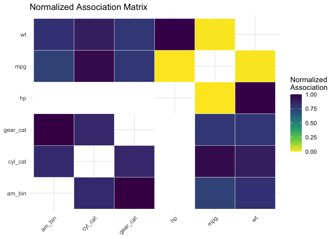
4.6 Normalization and Comparability
Different measures operate on different scales. Some are naturally bounded to \([0, 1]\); others are unbounded. To compare associations across variable pairs, we often need to normalize.
4.6.1 Standard Normalization Approaches
Min-max scaling: Scale a measure to \([0, 1]\) using its theoretical bounds \[\text{Normalized} = \frac{\text{Measure} - \min}{\max - \min}\]
Absolute value: For measures that can be negative (e.g., correlation), use absolute value if directionality is not of interest \[\text{Normalized} = |\text{Measure}|\]
Fisher z-transformation: For Pearson’s \(r\) specifically, use \(z = \frac{1}{2} \ln\left(\frac{1+r}{1-r}\right)\) to stabilize variance
Mutual information normalization: Divide by maximum possible MI or entropy \[\text{Normalized MI} = \frac{I(X;Y)}{\min(H(X), H(Y))}\]
4.6.2 Important Caveats
Normalization enables ranking but not direct comparison across measure types. A normalized value of 0.6 for Cramér’s V is not equivalent to 0.6 for Spearman’s \(\rho\). It helps to:
Document your normalization choice
Interpret results within measure families first
Use normalization to identify anomalies and ranking, not to claim equivalence
# Example: normalize association matrix to [0, 1]assoc_matrix_norm <- assoc_matrixdiag(assoc_matrix_norm) <-NA# Exclude diagonal (all 1s)# Normalize each off-diagonal valuemin_assoc <-min(assoc_matrix_norm, na.rm =TRUE)max_assoc <-max(assoc_matrix_norm, na.rm =TRUE)assoc_matrix_norm <- (assoc_matrix_norm - min_assoc) / (max_assoc - min_assoc)diag(assoc_matrix_norm) <-1# Restore diagonal# Heatmap of normalized valuesassoc_matrix_norm |>as.data.frame() |> tibble::rownames_to_column(var ="x") |>pivot_longer(-x, names_to ="y", values_to ="assoc") |>filter(x != y) |># Exclude diagonal for clarityggplot(aes(x = x, y = y, fill = assoc)) +geom_tile(color ="white") +scale_fill_viridis_c(direction =-1, na.value ="white") +labs(title ="Normalized Association Matrix",x =NULL, y =NULL, fill ="Normalized\nAssociation" ) +theme_minimal() +theme(axis.text.x =element_text(angle =45, hjust =1))
4.7 Handling Special Cases
4.7.1 Missing Data
Associations with missing data require explicit handling:
Listwise deletion: Remove all rows with any missing values (simple but wasteful)
Pairwise deletion: Compute each association only from complete cases for that pair (more data, but samples vary by pair)
Imputation: Replace missing values with estimates before computing associations
Here is a step-by-step workflow for building a unified association matrix:
Classify variables by type (continuous, discrete, ordinal, categorical, binary)
Handle missing data explicitly (document your choice)
Inspect distributions for outliers, skewness, and multimodality
Select measures based on the type-aware selection matrix above
Compute pairwise associations with appropriate measures
Normalize if comparability across pairs is desired
Visualize as a heatmap or network (see later chapters)
Interpret in context (avoid overstating quantitative results)
4.9 Summary and Key Takeaways
Variable types matter: Different measurement scales require different association measures to avoid misleading results.
Classical measures (Pearson, Spearman, Cramér’s V, \(\eta^2\)) are efficient, interpretable, and widely understood, but each is specialized for specific type combinations.
Modern alternatives (distance correlation, MIC, mutual information) offer greater flexibility and can detect nonlinear relationships, but are often more computationally expensive and less interpretable.
Type-aware framework: A systematic approach to selecting appropriate measures based on variable type combinations ensures valid and comparable association estimates.
Normalization enables ranking but does not erase conceptual differences between measures. It helps to document our choices and interpret results carefully.
Special cases (missing data, outliers) require explicit handling. Rank-based measures are more robust than Pearson correlation to outliers.
4.10 Looking Ahead
With a unified framework for association measurement now in hand, the next chapter extends this work to nonlinear and conditional associations. We plan to explore copulas, partial correlations, and graphical models to capture more complex dependence structures. Then, we move to network representations that visualize multivariate association patterns in a format that stakeholders can interpret and act upon.
Anderson, T. W. 1985. “An Introduction to Multivariate Statistical Analysis, 2nd Edition.”Biometrics 41 (3): 815. https://doi.org/10.2307/2531310.
David, F. N., and H. Cramer. 1947. “Mathematical Methods of Statistics.”Biometrika 34 (3/4): 374. https://doi.org/10.2307/2332454.
Fisher, Sir Ronald A. 1990. “Statistical Methods for Research Workers.”Statistical Methods, Experimental Design, and Scientific Inference. Oxford University PressOxford. https://doi.org/10.1093/oso/9780198522294.002.0003.
Pearson, Karl. 1895. “VII. Note on Regression and Inheritance in the Case of Two Parents.”Proceedings of the Royal Society of London 58 (347–352): 240–42. https://doi.org/10.1098/rspl.1895.0041.
Reshef, David N., Yakir A. Reshef, Hilary K. Finucane, Sharon R. Grossman, Gilean McVean, Peter J. Turnbaugh, Eric S. Lander, Michael Mitzenmacher, and Pardis C. Sabeti. 2011. “Detecting Novel Associations in Large Data Sets.”Science 334 (6062): 1518–24. https://doi.org/10.1126/science.1205438.
Sklar, M. 1959. “Fonctions de répartition à n Dimensions Et Leurs Marges.” In Annales de l’ISUP, 8:229–31. 3.
Spearman, C. 1961. “The Proof and Measurement of Association Between Two Things.” In Studies in Individual Differences: The Search for Intelligence., 45–58. Appleton-Century-Crofts. https://doi.org/10.1037/11491-005.
Székely, Gábor J., Maria L. Rizzo, and Nail K. Bakirov. 2007. “Measuring and Testing Dependence by Correlation of Distances.”The Annals of Statistics 35 (6). https://doi.org/10.1214/009053607000000505.