7  Interactive Exploration with Shiny

7.1 Introduction: The Limitations of Static Visualization

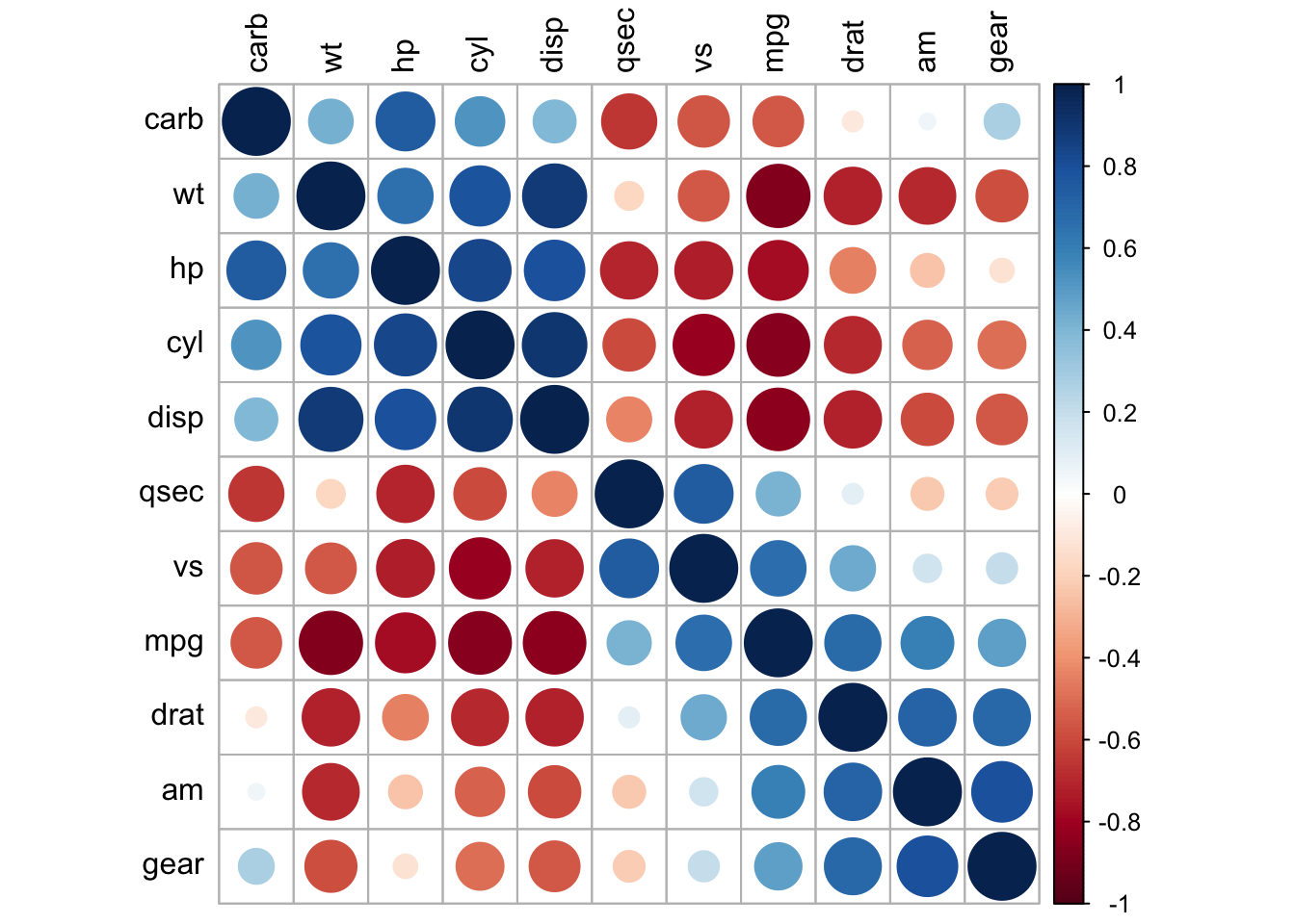
In previous chapters, we computed association matrices, created correlation heatmaps, and drew network graphs. These static visualizations are publication-ready and reproducible, but they can be inherently limited: each figure represents one choice of parameters, one threshold, one layout, one subset of data.

Consider a researcher working with network data:

• A network visualization is created with a threshold of 0.5. But what happens at 0.6? Or 0.4?
• One layout algorithm reveals a community structure. Does the Louvain algorithm find the same communities as Leiden?
• A variable appears central in the full dataset. But how important is it in a particular subgroup?

Static analysis answers one question at a time. Each new question typically requires code modification, recomputation, and a new figure.

Interactive analysis can empower exploration. Users can adjust parameters, filter data, and compare perspectives without waiting for recomputation, enabling discovery of patterns that static workflows often miss.

This chapter introduces Shiny, an R web framework that can transform exploratory analysis from a batch workflow into an interactive conversation with data. Rather than asking “what does this plot show?”, interactive tools let practitioners ask “what if I change this parameter?” or “how does this look in this subgroup?” and receive near-instant visual feedback.

7.2 Part I: Principles of Interactive Data Exploration

7.2.1 The Problem with Single Summaries

A single figure is frozen in time and parameter space. Consider a correlation matrix visualization:

# Static correlation heatmap - one view only
data(mtcars)
cor_mtcars <- cor(mtcars)

# Choose one color scheme, one ordering, one threshold
corrplot(cor_mtcars, method = "circle", order = "hclust", 
         tl.col = "black")

This figure effectively communicates the correlation structure, but:

1. No threshold filtering: The plot shows all correlations, including weak ones
2. No subset comparison: You cannot quickly examine correlations for sedans vs. sports cars
3. No parameter exploration: What if the clustering order were different?
4. No interaction: Hovering over cells, highlighting related variables, or zooming is impossible

Practitioners often resort to creating multiple figures to show different perspectives, one for each threshold, subgroup, or parameter choice. This multiplies the number of static outputs and makes comparison harder, not easier.

7.2.2 Benefits of Interactivity

Interactive tools address these limitations by enabling:

1. Real-time parameter adjustment: Change a threshold and watch the network update instantly
2. Dynamic subsetting: Filter data by group or criteria without restarting the analysis
3. Hover interactions: Explore details on demand (e.g., exact correlation values, variable names)
4. Cross-linked views: Highlight a node in a network and see its correlations in a table
5. No computation overhead: After the initial render, interactions are nearly instantaneous

These capabilities can transform exploration from passive viewing to active interrogation.

7.2.3 When Interactive Tools Matter Most

Interactive exploration is most valuable when:

• Parameter sensitivity is high: Small changes in thresholds or algorithms yield very different results
• Subgroup heterogeneity exists: Patterns differ across demographic or categorical groups
• Stakeholders are non-technical: Interactive tools make findings accessible without requiring coding
• The data are high-dimensional: Static visualizations of 50+ variables become unreadable; interactivity allows focus on relevant subsets
• Iterative discovery is the goal: Rather than hypothesis testing, you are searching for patterns

Conversely, we still need static visualizations for publication and presentation, where reproducibility and editorial control matter more than exploration.

7.3 Part II: Introduction to Shiny

7.3.1 Shiny Basics: UI and Server

Shiny separates an application into two components:

1. User Interface (UI): Layout, controls (sliders, dropdowns, buttons), and output placeholders
2. Server logic: Reactive computations that respond to user inputs

A minimal Shiny app has this structure:

library(shiny)

# Define UI
ui <- fluidPage(
  titlePanel("My First Shiny App"),
  sidebarLayout(
    sidebarPanel(
      sliderInput("threshold", "Correlation Threshold:", 
                  min = 0, max = 1, value = 0.5, step = 0.05)
    ),
    mainPanel(
      plotOutput("correlation_plot")
    )
  )
)

# Define server logic
server <- function(input, output) {
  output$correlation_plot <- renderPlot({
    # This code runs whenever input$threshold changes
    cor_mtcars <- cor(mtcars)
    # Create network based on current threshold
    adj <- (abs(cor_mtcars) > input$threshold) * 1
    diag(adj) <- 0
    # Create visualization...
  })
}

# Run the app
shinyApp(ui, server)

The key concept is that when a user adjusts the slider, the value in input$threshold updates, triggering a recomputation of output$correlation_plot.

7.3.2 Reactivity: The Heart of Shiny

Reactivity is Shiny’s mechanism for connecting inputs to outputs. A reactive expression recomputes only when its dependencies change:

server <- function(input, output) {
  # Reactive expression: computes only when threshold changes
  net_data <- reactive({
    cor_mtcars <- cor(mtcars)
    adj <- (abs(cor_mtcars) > input$threshold) * 1
    diag(adj) <- 0
    graph_from_adjacency_matrix(adj, mode = "undirected", weighted = TRUE)
  })
  
  # Outputs can depend on reactive expressions
  output$net_viz <- renderPlot({
    net <- net_data()
    plot(net)
  })
  
  output$summary_stats <- renderTable({
    net <- net_data()
    tibble(
      Metric = c("Nodes", "Edges", "Density"),
      Value = c(vcount(net), ecount(net), edge_density(net))
    )
  })
}

Notice: net_data() is defined once but used in multiple outputs. Both outputs automatically update together when input$threshold changes. This dependency tracking is automatic in Shiny (you need not explicitly code update sequences).

7.3.3 Common UI Input Controls

Shiny provides many input types:

# Slider for continuous values
sliderInput("threshold", "Threshold:", min = 0, max = 1, value = 0.5)

# Select dropdown for choices
selectInput("variable", "Variable:", choices = c("x1", "x2", "x3"))

# Radio buttons for mutually exclusive options
radioButtons("method", "Method:", 
             choices = c("Pearson", "Spearman", "Kendall"))

# Checkbox for binary options
checkboxInput("show_labels", "Show node labels", value = TRUE)

# Multiple selection
selectInput("subgroups", "Filter by group:", 
            choices = unique(data$group), 
            multiple = TRUE)

# Date range picker
dateRangeInput("date_range", "Select date range:", 
               start = "2020-01-01", end = "2023-12-31")

7.3.4 Common Output Types

Similarly, outputs can render various visualizations and tables:

# Plot output
plotOutput("myplot")

# Table output
tableOutput("mytable")
# or for prettier tables:
dataTableOutput("interactive_table")

# Text output
textOutput("summary_text")

# HTML output (for custom formatting)
htmlOutput("custom_html")

# UI output (dynamically generated controls)
uiOutput("dynamic_controls")

7.4 Part III: Interactive Association Exploration

7.4.1 Example: Threshold Explorer

Let us build a practical interactive tool that explores how network structure changes as the correlation threshold varies:

library(shiny)
library(igraph)
library(tidygraph)
library(ggraph)
library(ggplot2)
library(dplyr)

ui <- fluidPage(
  titlePanel("Correlation Network Threshold Explorer"),
  sidebarLayout(
    sidebarPanel(
      sliderInput("threshold", 
                  "Correlation Threshold:", 
                  min = 0, max = 1, value = 0.5, step = 0.05),
      helpText("Adjust to see how network structure changes."),
      br(),
      downloadButton("downloadPlot", "Download Plot")
    ),
    mainPanel(
      tabsetPanel(
        tabPanel("Network Visualization",
                 plotOutput("network_plot", height = "600px")),
        tabPanel("Network Statistics",
                 tableOutput("network_stats")),
        tabPanel("Correlation Distribution",
                 plotOutput("cor_distribution"))
      )
    )
  )
)

server <- function(input, output, session) {
  # Reactive network data
  net_reactive <- reactive({
    cor_mtcars <- cor(mtcars)
    adj <- (abs(cor_mtcars) > input$threshold) * 1
    diag(adj) <- 0
    graph_from_adjacency_matrix(adj, mode = "undirected", weighted = TRUE)
  })
  
  # Network plot
  output$network_plot <- renderPlot({
    net <- net_reactive()
    net_tidy <- as_tbl_graph(net)
    
    ggraph(net_tidy, layout = 'fr') +
      geom_edge_link(edge_colour = "gray60", alpha = 0.5) +
      geom_node_point(size = 5, colour = "steelblue") +
      geom_node_text(aes(label = name), repel = TRUE, size = 3) +
      labs(title = paste("Network at Threshold =", input$threshold)) +
      theme_void()
  })
  
  # Network statistics table
  output$network_stats <- renderTable({
    net <- net_reactive()
    tibble(
      Metric = c("Nodes", "Edges", "Density", "Average Degree", "Diameter"),
      Value = c(
        vcount(net),
        ecount(net),
        round(edge_density(net), 3),
        round(mean(degree(net)), 3),
        ifelse(ecount(net) > 0, diameter(net), NA)
      )
    )
  }, striped = TRUE, bordered = TRUE)
  
  # Distribution of all correlations
  output$cor_distribution <- renderPlot({
    cor_mtcars <- cor(mtcars)
    cor_values <- cor_mtcars[upper.tri(cor_mtcars)]
    
    ggplot(tibble(correlation = cor_values), aes(x = correlation)) +
      geom_histogram(bins = 20, fill = "steelblue", alpha = 0.7) +
      geom_vline(xintercept = input$threshold, colour = "red", linetype = "dashed", size = 1) +
      geom_vline(xintercept = -input$threshold, colour = "red", linetype = "dashed", size = 1) +
      labs(title = "Distribution of All Correlations",
           subtitle = "Red lines show current threshold",
           x = "Correlation", y = "Frequency") +
      theme_minimal()
  })
  
  # Download handler
  output$downloadPlot <- downloadHandler(
    filename = function() {
      paste0("network_threshold_", input$threshold, ".png")
    },
    content = function(file) {
      png(file, width = 800, height = 600)
      net <- net_reactive()
      net_tidy <- as_tbl_graph(net)
      plot(ggraph(net_tidy, layout = 'fr') +
             geom_edge_link(edge_colour = "gray60", alpha = 0.5) +
             geom_node_point(size = 5, colour = "steelblue") +
             geom_node_text(aes(label = name), repel = TRUE) +
             theme_void())
      dev.off()
    }
  )
}

shinyApp(ui, server)

7.4.2 Example: Subgroup Comparison

Interactive tools excel at comparing patterns across subgroups. Here is an application that compares correlation networks across iris species:

ui <- fluidPage(
  titlePanel("Iris Network by Species"),
  sidebarLayout(
    sidebarPanel(
      selectInput("species", "Select Species:", 
                  choices = unique(iris$Species)),
      sliderInput("threshold", 
                  "Correlation Threshold:", 
                  min = 0, max = 1, value = 0.5, step = 0.05),
      radioButtons("layout", "Graph Layout:",
                   choices = c("Force-Directed" = "fr", 
                              "Circle" = "circle"))
    ),
    mainPanel(
      plotOutput("species_network", height = "600px"),
      br(),
      tableOutput("centrality_table")
    )
  )
)

server <- function(input, output, session) {
  # Filter data by species
  species_data <- reactive({
    iris |>
      filter(Species == input$species) |>
      select(-Species)
  })
  
  # Compute network for selected species
  species_net <- reactive({
    data <- species_data()
    cor_mat <- cor(data)
    adj <- (abs(cor_mat) > input$threshold) * 1
    diag(adj) <- 0
    graph_from_adjacency_matrix(adj, mode = "undirected", weighted = TRUE)
  })
  
  # Plot network with user-selected layout
  output$species_network <- renderPlot({
    net <- species_net()
    net_tidy <- as_tbl_graph(net)
    
    layout_func <- if (input$layout == "fr") {
      "fr"
    } else {
      "circle"
    }
    
    ggraph(net_tidy, layout = layout_func) +
      geom_edge_link(edge_colour = "gray60", alpha = 0.6) +
      geom_node_point(size = 6, colour = "coral") +
      geom_node_text(aes(label = name), repel = TRUE, size = 4) +
      labs(title = paste("Network for", input$species)) +
      theme_void()
  })
  
  # Node centrality measures
  output$centrality_table <- renderTable({
    net <- species_net()
    tibble(
      Variable = names(species_data()),
      Degree = degree(net),
      Betweenness = round(betweenness(net), 2),
      Closeness = round(closeness(net), 3)
    ) |>
      arrange(desc(Degree))
  }, striped = TRUE)
}

shinyApp(ui, server)

7.5 Part IV: Performance and Reactive Programming Patterns

7.5.1 Avoiding Redundant Computation

As apps grow complex, they can become slow if computations repeat unnecessarily. The solution is strategic use of reactive expressions:

# Bad: Correlations computed twice
server <- function(input, output) {
  output$heatmap <- renderPlot({
    cor_data <- cor(mtcars)  # Computed here
    # plot heatmap
  })
  
  output$network <- renderPlot({
    cor_data <- cor(mtcars)  # Computed again!
    # plot network
  })
}

# Good: Correlations computed once, reused
server <- function(input, output) {
  cor_reactive <- reactive({
    cor(mtcars)
  })
  
  output$heatmap <- renderPlot({
    cor_data <- cor_reactive()  # Uses cached result
    # plot heatmap
  })
  
  output$network <- renderPlot({
    cor_data <- cor_reactive()  # Reuses same result
    # plot network
  })
}

7.5.2 Debouncing and Lazy Evaluation

Some inputs change very rapidly (e.g., a slider dragged quickly). Without debouncing, Shiny recomputes on every drag. Solutions include:

# Debounce: only recompute 0.5 seconds after slider stops moving
threshold_debounced <- debounce(reactive(input$threshold), 500)

server <- function(input, output) {
  output$plot <- renderPlot({
    # Uses debounced threshold; only recomputes after user stops dragging
    threshold <- threshold_debounced()
    # ... plot code ...
  })
}

# Alternatively, use an "Apply" button to batch updates
server <- function(input, output) {
  apply_button <- eventReactive(input$apply_button, {
    list(threshold = input$threshold, 
         species = input$species)
  })
  
  output$plot <- renderPlot({
    params <- apply_button()  # Only recomputes when button is clicked
    # ... plot code ...
  })
}

7.5.3 Conditional Panels

Apps often need dynamic UI: show certain controls only when relevant. Shiny provides conditionalPanel():

ui <- fluidPage(
  sidebarPanel(
    selectInput("plot_type", "Plot Type:", 
                choices = c("Network", "Heatmap", "Scatter")),
    
    # Show network options only when "Network" is selected
    conditionalPanel(
      condition = "input.plot_type == 'Network'",
      sliderInput("threshold", "Threshold:", min = 0, max = 1, value = 0.5),
      radioButtons("layout", "Layout:", 
                   choices = c("fr", "circle", "spring"))
    ),
    
    # Show heatmap options only when "Heatmap" is selected
    conditionalPanel(
      condition = "input.plot_type == 'Heatmap'",
      radioButtons("heatmap_method", "Distance Method:", 
                   choices = c("euclidean", "correlation"))
    )
  ),
  mainPanel(
    plotOutput("main_plot")
  )
)

7.6 Part V: Design Principles for Interactive Exploration Tools

7.6.1 Principle 1: Progressive Disclosure

Users can be overwhelmed by too many options at once. It helps to group controls logically and use tabs or collapsible panels:

ui <- fluidPage(
  tabsetPanel(
    tabPanel("Data Overview",
             # Simple view: just load and show data
             fileInput("data_file", "Choose CSV"),
             tableOutput("data_preview")),
    
    tabPanel("Exploration",
             # Intermediate view: threshold, subset options
             sliderInput("threshold", "Threshold:", 0, 1, 0.5)),
    
    tabPanel("Advanced",
             # Advanced view: algorithms, layouts, statistics
             radioButtons("algorithm", "Algorithm:", ...),
             radioButtons("layout", "Layout:", ...))
  )
)

7.6.2 Principle 2: Instant Feedback

Users often benefit from immediate visual feedback. Try to avoid long computations. Instead:

• Precompute expensive steps (e.g., large network layouts) at app startup
• Use withProgress() to show a progress bar for longer operations
• Debounce rapid input changes

7.6.3 Principle 3: Clarity Over Features

Too many controls can confuse users. Consider prioritizing:

1. Essential controls: What do users want to change first?
2. Sensible defaults: Pre-populate with reasonable starting values
3. Documentation: Include help text explaining each control

7.6.4 Principle 4: Comparison Facilitates Discovery

When comparing across subgroups or time periods, arrange views side-by-side or with linked highlighting:

ui <- fluidPage(
  fluidRow(
    column(6, h3("Species A"), plotOutput("net_a")),
    column(6, h3("Species B"), plotOutput("net_b"))
  )
)

7.7 Part VI: Limitations of Interactive Tools

While powerful, interactive exploration has drawbacks:

1. Reproducibility: Interactive explorations are harder to document than scripts. Always maintain an underlying analysis script.
2. Scalability: Real-time computation works only for moderately large datasets. Networks with 10,000+ nodes often require pre-computation or sampling.
3. Learning curve: Non-technical users need training to use interactive apps effectively.
4. Maintenance burden: Apps require hosting and updates; static reports are simpler to archive.

Best practice: Use interactive tools for exploration, then document findings in static reports.

7.8 Part VII: From Principles to Practice

The chapters so far have built the foundation for association analysis:

• Chapters 1-3: Data types and univariate/bivariate summaries
• Chapter 4: Association measures for mixed types
• Chapter 5: Nonlinear and conditional associations
• Chapter 6: Network representations
• Chapter 7: Interactive exploration (this chapter)

Now we integrate all these components into a cohesive, interactive tool. The next chapter introduces AssociationExplorer, a Shiny application designed specifically for exploratory association analysis. AssociationExplorer combines:

• Flexible association measures: Automatically select appropriate measures for mixed-type data
• Interactive parameter adjustment: Threshold, community detection algorithms, layouts
• Multiple linked views: Network, correlation matrix, summary statistics, and variable details
• Data filtering and subgrouping: Explore associations for specific observations or categories
• Publication-ready export: Save visualizations and data summaries

AssociationExplorer demonstrates how the principles and techniques from this chapter, combined with sound statistical practice and user-centered design, enable practitioners to explore high-dimensional association structures interactively, discover patterns that static analysis would miss, and communicate findings effectively to diverse audiences.

7.9 Summary and Key Takeaways

• Static analysis freezes findings in parameter space: Each figure answers one specific question; new questions require recoding.
• Interactive tools enable iterative discovery: Parameters adjust in real-time, subsets filter instantly, and multiple views stay synchronized.
• Shiny separates UI and server logic: Inputs drive outputs through reactive expressions that automatically track dependencies.
• Reactivity is central to Shiny’s power: Declaring dependencies once means outputs update together without explicit orchestration.
• Performance requires strategic caching: Use reactive expressions to compute expensive operations once and reuse results.
• Good interactive tools follow design principles: Progressive disclosure, instant feedback, clarity, and comparison-oriented layouts make exploration intuitive.
• Interactive and static methods are complementary: Use interactivity for exploration, static reports for communication.

7.10 Looking Ahead

With Shiny principles established, we now turn to a complete, production-ready application: AssociationExplorer. The following chapter showcases how these principles integrate into a comprehensive tool for exploring, understanding, and communicating association structures in complex tabular data.