17.1 Introduction: From Local Explanations to Automated Model Search
In the previous chapters, we moved from global summaries to local additive explanations. We now take a complementary step and consider how model construction itself can be partially automated, while still serving descriptive goals.
AutoML (automated machine learning) refers to the use of algorithms to automate parts of the model building process, such as trying multiple model types, tuning hyperparameters, and ranking candidates with a common evaluation metric. It is often presented as a performance oriented engineering workflow. That view is useful, but in descriptive analysis we can also treat AutoML as a structured instrument for learning about data. By exploring multiple model families and hyperparameters under a common evaluation protocol, we obtain a comparative map of predictive structure.
This chapter develops that perspective. We formalize the main ingredients of AutoML, implement a reproducible search workflow in R, and discuss how to interpret AutoML outputs in a careful descriptive way. We also revisit the same logic through two production platforms, Vertex AI AutoML (Google Cloud Console) and SageMaker Canvas (Amazon Web Services), to illustrate how these ideas are operationalized in common no-code and low-code environments. The objective is not to replace domain reasoning with automation, but to use automation to support transparent and technically grounded model comparison.
17.2 Why AutoML Can Be Useful for Descriptive Analysis
When we fit one model at a time, we often learn deeply about that model, but we can miss broader patterns. A modest AutoML workflow helps us answer additional questions:
does a flexible nonlinear model materially outperform a simpler baseline,
how sensitive performance is to hyperparameter choices,
whether several candidate models are practically tied,
how robust model rankings are across resamples.
These are descriptive questions about predictive structure and model behavior under the observed data distribution. As in earlier chapters, they should not be interpreted as causal claims.
17.3 AutoML as an Optimization Problem
A generic AutoML procedure searches over a space of pipelines and minimizes an estimated generalization loss.
Let \(\mathcal{A}\) denote a set of algorithms, and let \(\Lambda_a\) be the hyperparameter space for algorithm \(a \in \mathcal{A}\). A candidate is a pair \((a, \lambda)\) with \(\lambda \in \Lambda_a\). For loss function \(L\), the target can be written as (Feurer et al. 2019; Automated Machine Learning: Methods, Systems, Challenges 2019):
We reserve a final test set and perform model search only on analysis_data. This separation helps us avoid optimistic reporting when comparing many candidates.
17.5 A Reproducible Search and Evaluation Engine
We now define helper functions for fold creation, RMSE computation, and candidate evaluation.
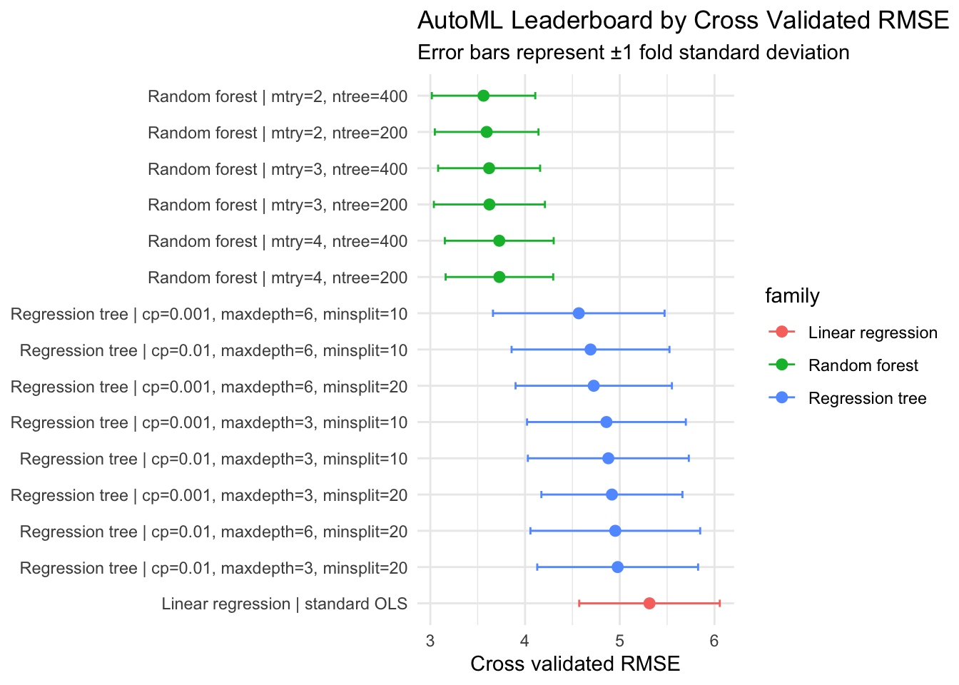
The leaderboard provides more than a winner. It shows whether performance differences are large, modest, or practically negligible relative to resampling variability.
17.7 Selecting a Final Candidate and Evaluating on Holdout Data
We now fit the best ranked candidate on all analysis_data and evaluate once on the untouched test set.
The gap between cross validated and holdout RMSE offers a quick diagnostic of selection stability. A small gap suggests that the search process did not overfit strongly to resampling noise.
17.8 Near Optimal Models and Practical Equivalence
A useful descriptive habit is to avoid over interpreting tiny leaderboard differences. One pragmatic criterion is to treat candidates as near optimal when their mean RMSE is within one standard deviation of the best candidate.
When several models are near tied, we can use secondary criteria, for example, computational cost, interpretability, or robustness under distribution shift assumptions.
17.9 Descriptive Interpretation of AutoML Results
In a descriptive workflow, the AutoML output is not only a model selector. It is also a structured summary of what the data seem to support under competing functional assumptions.
For instance:
if linear regression is competitive, the dominant structure may be close to additive linear signal,
if trees and forests improve substantially, nonlinearities or interactions likely matter,
if many configurations tie, model uncertainty should be communicated explicitly.
This interpretation remains predictive and data dependent. As discussed earlier in the book, moving from predictive regularities to causal statements requires additional design assumptions and identification strategies.
17.10 Good Practice for Reporting AutoML in Descriptive Work
To keep reporting transparent and reproducible, it is often useful to document:
search space (model families and hyperparameter ranges),
resampling protocol and random seeds,
optimization metric and any tie breaking rule,
final holdout performance,
whether conclusions rely on one model or a near optimal set.
These elements help readers understand how much of the final conclusion is driven by data signal versus search design.
17.11 Limits and Cautions
AutoML can improve coverage of model space, but it does not eliminate substantive judgment.
Key limits include:
performance metrics can hide subgroup specific errors,
search spaces can encode strong implicit priors,
correlated predictors can produce unstable model rankings,
repeated experimentation can still induce selection bias if holdout data are reused.
A careful descriptive workflow therefore combines automation with explicit diagnostics, domain context, and communication of uncertainty.
17.12 AutoML in Practice: Vertex AI and SageMaker Canvas
The R workflow above makes each modeling choice explicit. In practice, many teams implement similar logic through managed platforms. To connect this chapter to operational settings, we briefly consider two widely used platforms, Vertex AI AutoML and SageMaker Canvas, using the same evaluative lens developed earlier in the chapter.
17.12.1 Overview of Vertex AI AutoML
Vertex AI AutoML is Google’s managed environment for automated model training and selection. In tabular settings, it supports supervised tasks such as classification and regression by combining data preparation steps, candidate model search, hyperparameter tuning, and evaluation reporting within one workflow.
The platform workflow typically follows these steps:
users upload tabular data and specify the prediction target;
the system performs automatic data exploration and feature engineering;
candidates are generated by trying multiple model architectures and hyperparameter combinations;
each candidate is evaluated via cross-validation on a held-out portion of training data;
a leaderboard ranks models by performance metrics such as RMSE (regression) or AUC-ROC (classification);
the top-ranked model or an ensemble is deployed for inference.
Vertex AI emphasizes broad model exploration and provides strong predictive results, especially when sufficient computational budget is available. The platform generates detailed evaluation reports including feature importance scores and model comparison tables that align with the leaderboard concept discussed in this chapter.
17.12.2 Overview of SageMaker Canvas
SageMaker Canvas is AWS’s visual interface for building machine learning models with limited coding. For tabular data, it offers guided workflows for data ingestion, model building, evaluation, and prediction generation, with optional quick build versus standard optimization modes.
The Canvas workflow is similarly structured:
users import data via the web interface or cloud storage;
the system performs exploratory data analysis and data profiling;
the user specifies the target variable and builds a model with minimal configuration;
Canvas automatically tries different model families and hyperparameters;
results including predictions, model metrics, and feature importance are presented in a dashboard;
predictions can be generated on new data directly within the interface.
SageMaker Canvas prioritizes usability and rapid iteration. In applied contexts, this design can lower entry barriers for analysts who need interpretable summaries and quick feedback before investing in heavier engineering pipelines. The platform includes model explanation features that communicate variable importance to non-technical stakeholders.
17.12.3 Practical Comparison
Comparing Vertex AI AutoML and SageMaker Canvas from a descriptive analysis perspective highlights several structural patterns.
Similarities include:
both platforms automate model selection and hyperparameter tuning from tabular data,
both report standard evaluation metrics and feature importance summaries,
both allow prediction generation without manual pipeline coding,
both maintain a candidate leaderboard or ranking of explored models.
Structural differences documented in official platform descriptions include:
Vertex AI’s architecture is designed to explore a broader search space and can generate ensemble models for higher predictive accuracy, at the cost of longer training time,
SageMaker Canvas emphasizes quick iteration with a “quick build” mode for rapid baseline models and a “standard build” mode for more thorough search, trading speed for computational cost control,
Canvas aims for a beginner-friendly visual interface with drag-and-drop data preparation,
Vertex AI and Canvas differ in their approach to uncertainty quantification; Vertex AI provides detailed training metrics and hyperparameter sensitivity reports, while Canvas focuses on prediction confidence intervals,
pricing models differ, with Vertex AI billed by training time and SageMaker Canvas based on model training duration and complexity.
These contrasts should be interpreted as reflecting different design priorities rather than universal rankings. Organization policies, existing cloud investments, team technical expertise, and project requirements all influence which platform is more suitable in practice.
17.12.4 Strengths, Limitations, and Use Cases
For advanced descriptive analysis of tabular data, a platform choice can be framed in terms of analytic priorities.
Vertex AI AutoML can be attractive when broader model search and comprehensive feature importance analysis are central goals, and when organization infrastructure already uses Google Cloud Platform.
SageMaker Canvas can be attractive when rapid iteration, visual collaboration with non-technical stakeholders, and AWS ecosystem integration are priorities.
In both platforms, automated outputs still require statistical interpretation, especially when predictors are correlated, classes are imbalanced, or subgroup performance differs.
An analytically balanced approach is therefore to treat these platforms as structured experimentation environments documented by official resources. They can accelerate candidate discovery and provide transparent leaderboards for model comparison, while inferential framing, diagnostic scrutiny, and domain interpretation remain human responsibilities.
17.12.5 Implications for Descriptive and Exploratory Analysis
From the perspective of this book, the main value of these platforms is not only faster model fitting. Their broader contribution is methodological: they make it easier to compare many predictive hypotheses under a consistent evaluation framework, capture that comparison in transparent leaderboards, and generate feature importance summaries at scale.
That capacity aligns directly with advanced descriptive analysis, where we use predictive tools to characterize pattern strength, nonlinear structure, interaction potential, and uncertainty in model choice. Vertex AI and SageMaker Canvas operationalize the leaderboard and ranking logic developed in the R workflow of this chapter. When used with careful interpretation of results and explicit documentation of search design, platform-based AutoML can complement the transparent R-first workflow developed earlier in this chapter.
17.13 Summary and Key Takeaways
AutoML can be used as a descriptive instrument, not only as a predictive optimizer.
A transparent search setup provides comparative evidence about functional form and model sensitivity.
Leaderboards are most informative when interpreted with variability and near tie structure.
Platform implementations such as Vertex AI AutoML and SageMaker Canvas extend this logic to operational settings, with trade-offs in accuracy, speed, usability, and cost that should be evaluated in context.
Final model selection should be paired with untouched holdout evaluation and explicit reporting choices.
Automation supports analysis, but it does not replace substantive interpretation.
17.14 Looking Ahead
This chapter used automation to search model and hyperparameter spaces. The next chapter extends that idea to the predictor space itself, where automated feature engineering helps us discover transformed variables and interaction candidates that can improve both predictive performance and descriptive resolution.
Automated Machine Learning: Methods, Systems, Challenges. 2019. The Springer Series on Challenges in Machine Learning. Springer International Publishing. https://doi.org/10.1007/978-3-030-05318-5.
Feurer, Matthias, Aaron Klein, Katharina Eggensperger, Jost Tobias Springenberg, Manuel Blum, and Frank Hutter. 2019. “Auto-Sklearn: Efficient and Robust Automated Machine Learning.” In Automated Machine Learning, 113–34. Springer International Publishing. https://doi.org/10.1007/978-3-030-05318-5_6.