16 Shapley Values and Additive Explanations

16.1 Introduction: From Functional Profiles to Local Additive Attribution

In the previous chapter, we examined partial dependence and ICE curves as tools for reading model behavior across feature values. That perspective is global and profile based, which makes it useful for understanding shape and heterogeneity.

Shapley value explanations address a complementary question. For a specific observation, how can we decompose the model prediction into additive feature contributions in a principled way? This local decomposition is often valuable when we want to connect broad model behavior to case specific interpretation.

In this chapter, we develop Shapley values from their game theoretic definition, discuss practical estimation in tabular settings, and implement a reproducible workflow in R. We also connect local attributions to global summaries, because descriptive practice often moves back and forth between these two levels.

16.2 Why Shapley Values Matter in Descriptive Analysis

In complex predictive models, local explanations help us understand why two observations with different predictions are separated by the model. Additive decompositions are particularly appealing because they map each prediction into interpretable components relative to a reference level.

For descriptive work, this supports several goals:

explaining individual predictions in a structured and comparable format,
auditing whether model behavior aligns with domain expectations,
aggregating local contributions into global relevance summaries,
communicating model behavior with transparent bookkeeping.

As in earlier interpretability chapters, these are predictive attributions, not causal effects. A positive contribution indicates that the model prediction moves upward relative to a baseline when the feature is incorporated under the chosen attribution definition.

16.3 Shapley Values as a Cooperative Game

Let \(M = \{1, \dots, p\}\) denote feature indices, and let \(v_x(S)\) be a value function that measures the expected prediction when only features in subset \(S\) are known for observation \(x\).

For feature \(j\), the Shapley value is (Shapley 1953; Lundberg and Lee 2017):

\[ \phi_j(x) = \sum_{S \subseteq M \setminus \{j\}} \frac{|S|!(p-|S|-1)!}{p!}\left[v_x(S \cup \{j\}) - v_x(S)\right]. \]

The weighting term averages marginal contributions of feature \(j\) over all possible feature ordering contexts. This symmetry is a central reason why Shapley values are often used for additive explanation.

Under a given value function definition, Shapley values satisfy familiar axiomatic properties:

Efficiency (local accuracy), contributions sum to prediction minus baseline,
Symmetry, features with identical marginal roles receive identical credit,
Dummy (missingness), features with no marginal effect receive zero contribution,
Additivity, attribution is linear across games.

These properties are mathematical guarantees for the specified game. In applications, the practical interpretation still depends on how \(v_x(S)\) is defined and estimated.

16.4 Choosing the Value Function in Tabular Data

Two common choices appear in practice.

Marginal (interventional style) value functions, where unknown features are integrated over a background distribution without conditioning on selected features.
Conditional value functions, where unknown features are integrated conditionally on selected features.

The marginal approach is often easier to compute and aligns with many software defaults, but it can evaluate feature combinations that are less realistic under strong dependence. The conditional approach can better respect feature dependence, but requires additional modeling assumptions.

To keep the workflow transparent and reproducible, we use a marginal Monte Carlo approximation in this chapter, with explicit discussion of its limits.

16.5 Running Example: Random Forest on Boston Housing

We continue the interpretability sequence with a random forest predicting medv from a compact set of predictors.

data(Boston, package = "MASS")

set.seed(123)
idx <- sample(seq_len(nrow(Boston)), size = 0.7 * nrow(Boston))
train <- Boston[idx, ]
test <- Boston[-idx, ]

predictors <- c("lstat", "rm", "ptratio", "indus", "nox", "crim")
rf_formula <- as.formula(paste("medv ~", paste(predictors, collapse = " + ")))

set.seed(123)
rf_fit <- randomForest(
    rf_formula,
    data = train,
    ntree = 500,
    mtry = 2,
    importance = TRUE
)

rf_pred <- predict(rf_fit, newdata = test)
rf_rmse <- sqrt(mean((test$medv - rf_pred)^2))

rf_rmse

[1] 3.5575

The RMSE gives context for subsequent interpretation. As discussed earlier in the book, explanatory summaries are typically more informative when the predictive model has useful signal.

16.6 Monte Carlo Approximation of Shapley Values

Exact Shapley values require averaging over all subsets, which scales exponentially with the number of predictors. For tabular models, permutation based Monte Carlo estimators are often used.

The function below estimates Shapley values for one observation by averaging marginal contributions across random feature orderings and random background rows.

predict_rf <- function(model, newdata) {
    as.numeric(predict(model, newdata = newdata))
}

shapley_single_mc <- function(model,
                             x,
                             background,
                             features,
                             predict_fn,
                             n_permutations = 300,
                             seed = 123) {
    set.seed(seed)

    contrib <- setNames(rep(0, length(features)), features)

    for (b in seq_len(n_permutations)) {
        perm <- sample(features)
        z <- background[sample(seq_len(nrow(background)), 1), features, drop = FALSE]

        current <- z
        pred_prev <- predict_fn(model, current)

        for (f in perm) {
            current[[f]] <- x[[f]]
            pred_new <- predict_fn(model, current)
            contrib[f] <- contrib[f] + (pred_new - pred_prev)
            pred_prev <- pred_new
        }
    }

    contrib / n_permutations
}

Next, we compute local attributions for one test observation and verify approximate local accuracy.

background <- train[, predictors, drop = FALSE]
baseline <- mean(predict_rf(rf_fit, background))

obs_id <- 10
x_obs <- test[obs_id, predictors, drop = FALSE]
pred_obs <- predict_rf(rf_fit, x_obs)

phi_obs <- shapley_single_mc(
    model = rf_fit,
    x = x_obs,
    background = background,
    features = predictors,
    predict_fn = predict_rf,
    n_permutations = 400,
    seed = 123
)

check_tbl <- tibble::tibble(
    quantity = c("Baseline", "Prediction", "Baseline + Sum(phi)", "Difference"),
    value = c(
        baseline,
        pred_obs,
        baseline + sum(phi_obs),
        pred_obs - (baseline + sum(phi_obs))
    )
)

check_tbl |>
    gt() |>
    cols_label(
        quantity = "Quantity",
        value = "Value"
    ) |>
    fmt_number(columns = value, decimals = 4)

Quantity	Value
Baseline	22.2935
Prediction	18.2458
Baseline + Sum(phi)	18.6192
Difference	−0.3734

The final row should be near zero, up to Monte Carlo approximation error.

16.7 Visualizing Local Contributions

A local decomposition is often easiest to read when contributions are ordered by absolute magnitude.

local_tbl <- tibble::tibble(
    feature = names(phi_obs),
    phi = as.numeric(phi_obs)
) |>
    arrange(desc(abs(phi)))

local_tbl |>
    gt() |>
    cols_label(
        feature = "Feature",
        phi = "Shapley contribution"
    ) |>
    fmt_number(columns = phi, decimals = 3)

Feature	Shapley contribution
rm	−2.230
ptratio	−1.252
indus	−0.431
crim	0.217
lstat	0.090
nox	−0.069

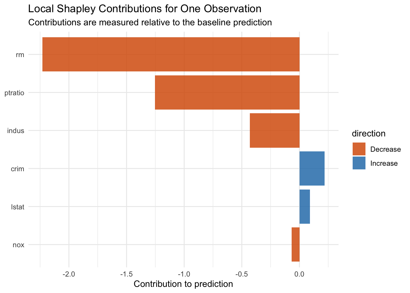
plot_tbl <- local_tbl |>
    mutate(
        direction = ifelse(phi >= 0, "Increase", "Decrease"),
        feature = factor(feature, levels = rev(feature))
    )

plot_tbl |>
    ggplot(aes(x = feature, y = phi, fill = direction)) +
    geom_col(alpha = 0.85) +
    coord_flip() +
    scale_fill_manual(values = c("Increase" = "#2c7fb8", "Decrease" = "#d95f0e")) +
    labs(
        title = "Local Shapley Contributions for One Observation",
        subtitle = "Contributions are measured relative to the baseline prediction",
        x = NULL,
        y = "Contribution to prediction"
    ) +
    theme_minimal()

Positive bars move the prediction above baseline, while negative bars move it below baseline. Reading contributions together with the original feature values helps preserve context.

value_context_tbl <- tibble::tibble(
    feature = predictors,
    feature_value = as.numeric(x_obs[1, predictors]),
    shapley = as.numeric(phi_obs[predictors])
)

value_context_tbl |>
    gt() |>
    cols_label(
        feature = "Feature",
        feature_value = "Observed value",
        shapley = "Shapley contribution"
    ) |>
    fmt_number(columns = c(feature_value, shapley), decimals = 3)

Feature	Observed value	Shapley contribution
lstat	11.690	0.090
rm	5.456	−2.230
ptratio	21.000	−1.252
indus	8.140	−0.431
nox	0.538	−0.069
crim	0.803	0.217

16.8 From Local to Global: Mean Absolute Shapley

A common global summary is the mean absolute contribution for each feature across many observations (Lundberg and Lee 2017):

\[ I_j^{SHAP} = \frac{1}{n}\sum_{i=1}^{n}|\phi_j(x_i)|. \]

This quantity is not a replacement for local analysis, but it provides a useful bridge between per case decomposition and global feature relevance.

shapley_many_mc <- function(model,
                           data,
                           background,
                           features,
                           predict_fn,
                           ids,
                           n_permutations = 250,
                           seed = 123) {
    res <- lapply(seq_along(ids), function(k) {
        i <- ids[k]
        phi_i <- shapley_single_mc(
            model = model,
            x = data[i, features, drop = FALSE],
            background = background,
            features = features,
            predict_fn = predict_fn,
            n_permutations = n_permutations,
            seed = seed + k
        )

        as.data.frame(as.list(phi_i)) |>
            mutate(obs_id = i)
    })

    bind_rows(res)
}

set.seed(999)
ids_explain <- sample(seq_len(nrow(test)), size = 40)

shap_values <- shapley_many_mc(
    model = rf_fit,
    data = test,
    background = background,
    features = predictors,
    predict_fn = predict_rf,
    ids = ids_explain,
    n_permutations = 300,
    seed = 300
)

global_shap <- tibble::tibble(
    feature = predictors,
    mean_abs_phi = sapply(predictors, function(v) mean(abs(shap_values[[v]])))
) |>
    arrange(desc(mean_abs_phi))

global_shap |>
    gt() |>
    cols_label(
        feature = "Feature",
        mean_abs_phi = "Mean |Shapley|"
    ) |>
    fmt_number(columns = mean_abs_phi, decimals = 3)

Feature	Mean \|Shapley\|
lstat	3.403
rm	3.074
ptratio	0.822
nox	0.603
indus	0.434
crim	0.302

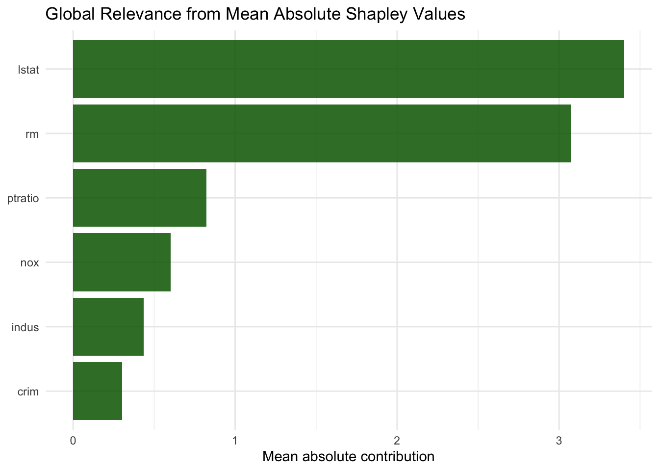
global_shap |>
    ggplot(aes(x = reorder(feature, mean_abs_phi), y = mean_abs_phi)) +
    geom_col(fill = "darkgreen", alpha = 0.85) +
    coord_flip() +
    labs(
        title = "Global Relevance from Mean Absolute Shapley Values",
        x = NULL,
        y = "Mean absolute contribution"
    ) +
    theme_minimal()

This summary can be compared with feature importance and partial dependence patterns from previous chapters. Agreement across methods often strengthens interpretation, while disagreement can signal dependence or interaction structure that deserves closer inspection.

16.9 Dependence Style View of a Shapley Feature

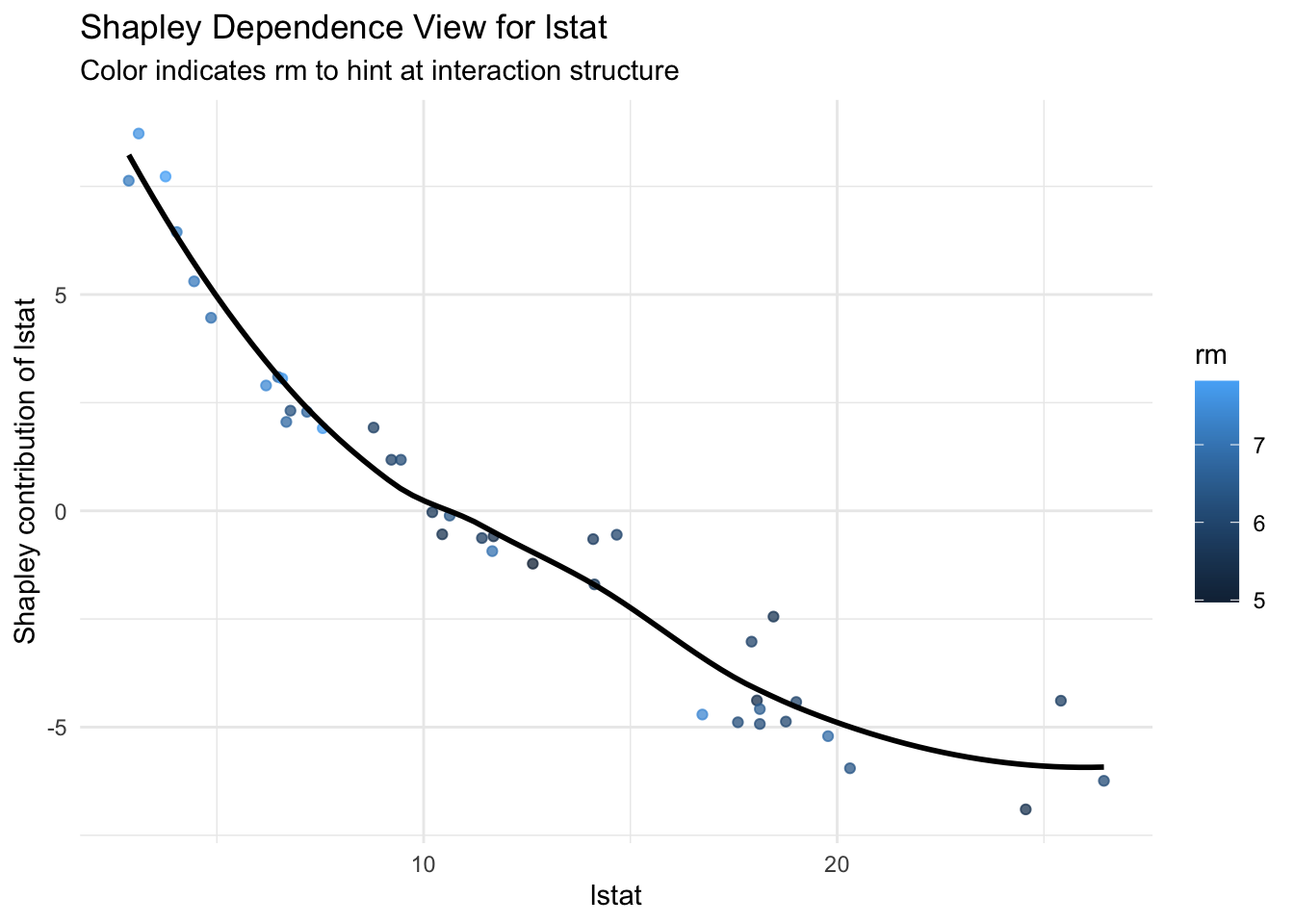
A practical diagnostic is to plot one feature against its Shapley contribution across observations. This helps us connect local attributions to profile style interpretation.

dep_tbl <- shap_values |>
    mutate(
        lstat_value = test$lstat[obs_id],
        rm_value = test$rm[obs_id]
    )

dep_tbl |>
    ggplot(aes(x = lstat_value, y = lstat, color = rm_value)) +
    geom_point(alpha = 0.75) +
    geom_smooth(method = "loess", se = FALSE, color = "black") +
    labs(
        title = "Shapley Dependence View for lstat",
        subtitle = "Color indicates rm to hint at interaction structure",
        x = "lstat",
        y = "Shapley contribution of lstat",
        color = "rm"
    ) +
    theme_minimal()

This display is not identical to PD or ICE, but it often reveals similar shape information and can highlight interaction patterns through the color gradient.

16.10 Practical Limitations and Interpretation Cautions

Shapley values provide a coherent additive decomposition, but interpretation remains conditional on modeling and estimation choices.

Dependence sensitivity. Under correlated predictors, attributions can shift when we change value function assumptions or background data.
Computational cost. Monte Carlo estimation can be expensive for large samples or many predictors.
Monte Carlo variability. Small contributions may fluctuate across runs when permutation counts are low.
Baseline dependence. Contributions are defined relative to a reference expectation, so absolute values depend on baseline choice.
Predictive attribution, not intervention. Contributions summarize model behavior, not causal response to manipulations.

In descriptive workflows, these limitations are manageable when we report assumptions explicitly and compare conclusions with complementary tools such as partial dependence and permutation importance.

16.11 Suggested Workflow for Robust Use

Building on the sequence of interpretability chapters so far, a practical workflow can be organized as follows:

establish predictive adequacy for the fitted model,
inspect global relevance summaries,
study profile based behavior with PD and ICE,
use Shapley values for case specific decomposition,
aggregate local contributions back to global summaries,
communicate assumptions and uncertainty about attribution.

This layered process balances readability with technical rigor, and helps avoid over interpreting any single explanation technique in isolation.

16.12 Summary and Key Takeaways

Shapley values extend the interpretability toolkit by providing additive local attributions with a clear mathematical foundation. The main points from this chapter are:

Shapley values decompose individual predictions relative to a baseline expectation.
Axiomatic properties support fairness style allocation of contribution credit for a specified value function.
Monte Carlo estimators make Shapley analysis practical in tabular models, with approximation error that can be monitored.
Mean absolute Shapley values provide a bridge to global relevance summaries across observations.
Interpretation quality depends on dependence assumptions, baseline choice, and computational settings.

Used jointly with profile and importance methods, Shapley explanations provide a detailed and communicable account of model behavior at both local and global scales.

16.13 Looking Ahead

The next chapter moves toward automated machine learning as a descriptive tool. With the interpretability components established in this part of the book, we can study how automated model search can be integrated with transparent diagnostics rather than treated as a purely black box procedure.