5  Extensions of Correlation: Nonlinear and Conditional

5.1 Introduction: Why Standard Correlation Falls Short

Pearson and Spearman correlations are powerful descriptive tools, but they capture only marginal associations (Pearson 1895; Anderson 1985; Spearman 1961). In real data, relationships often depend on context: a strong positive association for one subgroup may disappear or reverse in another. Additionally, standard correlations assume that relationships are linear (or at least monotonic), which can miss complex functional forms that drive patterns in nonlinear systems.

This chapter extends the correlation toolkit in two directions:

1. Nonlinear associations: Methods that detect and describe relationships that curve, oscillate, or follow other complex patterns
2. Conditional associations: Techniques that reveal how associations change across levels of other variables or contextual conditions

5.2 Part I: Nonlinear Association Methods

5.2.1 Visual Detection of Nonlinearity

Before applying formal measures, it helps to start with visual inspection. A scatterplot with a smooth trend line can reveal whether linearity is a reasonable assumption.

# Create dataset with various nonlinear relationships
set.seed(42)
n <- 200

nonlin_data <- tibble(
  Linear = seq(0, 10, length.out = n),
  Quadratic = seq(0, 10, length.out = n),
  Exponential = seq(0, 10, length.out = n),
  Sine = seq(0, 4 * pi, length.out = n),
  x_lin = rnorm(n, 0, 1),
  x_quad = rnorm(n, 0, 1),
  x_exp = rnorm(n, 0, 1),
  x_sin = rnorm(n, 0, 1)
) |>
  mutate(
    y_lin = Linear + x_lin,
    y_quad = 10 - Quadratic^2 / 8 + x_quad,
    y_exp = exp(Exponential / 3) + x_exp * 2,
    y_sin = sin(Sine) + x_sin
  )

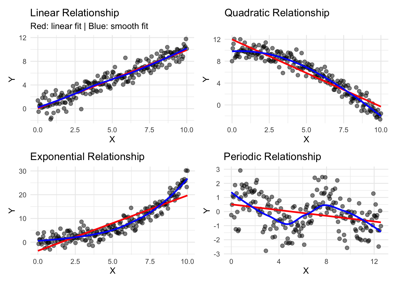
# Visualize multiple relationship types
p1 <- nonlin_data |>
  ggplot(aes(x = Linear, y = y_lin)) +
  geom_point(alpha = 0.5, size = 2) +
  geom_smooth(method = "lm", se = FALSE, color = "red", linewidth = 1) +
  geom_smooth(method = "loess", se = FALSE, color = "blue", linewidth = 1) +
  labs(
    title = "Linear Relationship",
    x = "X", y = "Y",
    subtitle = "Red: linear fit | Blue: smooth fit"
  ) +
  theme_minimal()

p2 <- nonlin_data |>
  ggplot(aes(x = Quadratic, y = y_quad)) +
  geom_point(alpha = 0.5, size = 2) +
  geom_smooth(method = "lm", se = FALSE, color = "red", linewidth = 1) +
  geom_smooth(method = "loess", se = FALSE, color = "blue", linewidth = 1) +
  labs(
    title = "Quadratic Relationship",
    x = "X", y = "Y"
  ) +
  theme_minimal()

p3 <- nonlin_data |>
  ggplot(aes(x = Exponential, y = y_exp)) +
  geom_point(alpha = 0.5, size = 2) +
  geom_smooth(method = "lm", se = FALSE, color = "red", linewidth = 1) +
  geom_smooth(method = "loess", se = FALSE, color = "blue", linewidth = 1) +
  labs(
    title = "Exponential Relationship",
    x = "X", y = "Y"
  ) +
  theme_minimal()

p4 <- nonlin_data |>
  ggplot(aes(x = Sine, y = y_sin)) +
  geom_point(alpha = 0.5, size = 2) +
  geom_smooth(method = "lm", se = FALSE, color = "red", linewidth = 1) +
  geom_smooth(method = "loess", se = FALSE, color = "blue", linewidth = 1) +
  labs(
    title = "Periodic Relationship",
    x = "X", y = "Y"
  ) +
  theme_minimal()

(p1 + p2) / (p3 + p4)

Interpretation: When the blue smooth curve (locally weighted scatterplot smoothing, LOESS) deviates substantially from the red linear fit, nonlinearity is present (Cleveland 1979). This visual diagnostic often provides helpful context before quantitative analysis.

5.2.2 Quantifying Nonlinearity: The \(R^2\) Contrast

A simple descriptive measure of nonlinearity is to compare the \(R^2\) from a linear model to the \(R^2\) from a smooth nonparametric model (such as LOESS or a spline):

\[\text{Nonlinearity Index} = R^2_{\text{smooth}} - R^2_{\text{linear}}.\]

The difference indicates how much variance can be explained by nonlinear structure that the linear model misses.

# Function to compute nonlinearity index
nonlinearity_index <- function(x, y) {
  df <- tibble(x = x, y = y) |>
    na.omit()
  
  # Linear model
  lm_fit <- lm(y ~ x, data = df)
  r2_linear <- summary(lm_fit)$r.squared
  
  # LOESS smooth fit
  loess_fit <- loess(y ~ x, data = df)
  r2_smooth <- 1 - (sum(loess_fit$residuals^2) / sum((df$y - mean(df$y))^2))
  
  tibble(
    R2_linear = r2_linear,
    R2_smooth = r2_smooth,
    Nonlinearity_Index = r2_smooth - r2_linear
  )
}

# Apply to our synthetic data
comparison <- bind_rows(
  nonlinearity_index(nonlin_data$Linear, nonlin_data$y_lin) |> 
    mutate(Relationship = "Linear"),
  nonlinearity_index(nonlin_data$Quadratic, nonlin_data$y_quad) |> 
    mutate(Relationship = "Quadratic"),
  nonlinearity_index(nonlin_data$Exponential, nonlin_data$y_exp) |> 
    mutate(Relationship = "Exponential"),
  nonlinearity_index(nonlin_data$Sine, nonlin_data$y_sin) |> 
    mutate(Relationship = "Periodic")
)

comparison |>
  gt() |>
  fmt_number(columns = c(R2_linear, R2_smooth, Nonlinearity_Index), decimals = 3)

R2_linear	R2_smooth	Nonlinearity_Index	Relationship
0.897	0.899	0.002	Linear
0.883	0.939	0.057	Quadratic
0.801	0.924	0.122	Exponential
0.095	0.284	0.189	Periodic

Interpretation: A high nonlinearity index can suggest that a linear model substantially underestimates the association strength. However, this measure is best paired with visual inspection, as sometimes the smooth fit overfits noise.

5.2.3 Distance Correlation: A Revisit with Nonlinearity in Focus

Recall from Chapter 4 that distance correlation detects both linear and nonlinear associations. Let’s examine how it performs on nonlinear data:

# Distance correlation comparison
library(energy)

comparison_dcor <- bind_rows(
  tibble(
    Relationship = "Linear",
    Pearson = cor(nonlin_data$Linear, nonlin_data$y_lin, method = "pearson"),
    Spearman = cor(nonlin_data$Linear, nonlin_data$y_lin, method = "spearman"),
    DistanceCorr = dcor(nonlin_data$Linear, nonlin_data$y_lin)
  ),
  tibble(
    Relationship = "Quadratic",
    Pearson = cor(nonlin_data$Quadratic, nonlin_data$y_quad, method = "pearson"),
    Spearman = cor(nonlin_data$Quadratic, nonlin_data$y_quad, method = "spearman"),
    DistanceCorr = dcor(nonlin_data$Quadratic, nonlin_data$y_quad)
  ),
  tibble(
    Relationship = "Exponential",
    Pearson = cor(nonlin_data$Exponential, nonlin_data$y_exp, method = "pearson"),
    Spearman = cor(nonlin_data$Exponential, nonlin_data$y_exp, method = "spearman"),
    DistanceCorr = dcor(nonlin_data$Exponential, nonlin_data$y_exp)
  ),
  tibble(
    Relationship = "Periodic",
    Pearson = cor(nonlin_data$Sine, nonlin_data$y_sin, method = "pearson"),
    Spearman = cor(nonlin_data$Sine, nonlin_data$y_sin, method = "spearman"),
    DistanceCorr = dcor(nonlin_data$Sine, nonlin_data$y_sin)
  )
)

comparison_dcor |>
  gt() |>
  fmt_number(columns = c(Pearson, Spearman, DistanceCorr), decimals = 3)

Relationship	Pearson	Spearman	DistanceCorr
Linear	0.947	0.955	0.946
Quadratic	−0.939	−0.942	0.947
Exponential	0.895	0.915	0.907
Periodic	−0.307	−0.315	0.332

Observation: Distance correlation captures all relationship types more uniformly than Pearson or Spearman, which may completely miss periodic patterns.

5.2.4 Generalized Additive Models (GAMs) for Smooth Associations

Generalized Additive Models extend linear regression by allowing smooth functions instead of linear terms (Hastie and Tibshirani 2017). For description, GAMs serve two purposes:

1. Visualize the functional form of a relationship
2. Quantify association strength via model diagnostics

# Fit GAM to exponential data
gam_fit <- gam(y_exp ~ s(Exponential), data = nonlin_data)

# Extract and visualize smooth term
plot_data <- tibble(
  Exponential = seq(min(nonlin_data$Exponential), 
                     max(nonlin_data$Exponential), 
                     length.out = 100)
)

# Predict from GAM
preds <- predict(gam_fit, newdata = plot_data, se.fit = TRUE)

plot_data <- plot_data |>
  mutate(
    fit = preds$fit,
    se = preds$se.fit,
    upper = fit + 1.96 * se,
    lower = fit - 1.96 * se
  )

# Visualize with original data
ggplot(nonlin_data, aes(x = Exponential, y = y_exp)) +
  geom_point(alpha = 0.4, size = 2) +
  geom_ribbon(data = plot_data, aes(y = fit, ymin = lower, ymax = upper),
              fill = "lightblue", color = NA, alpha = 0.5) +
  geom_line(data = plot_data, aes(y = fit), color = "darkblue", linewidth = 1) +
  labs(
    title = "GAM Smooth Term: Exponential Relationship",
    x = "X", y = "Y",
    subtitle = "Blue ribbon: 95% confidence band"
  ) +
  theme_minimal()

# Model summary
tibble(
  Metric = c("Deviance Explained", "GCV Score"),
  Value = c(
    paste0(round(summary(gam_fit)$dev.expl * 100, 1), "%"),
    round(gam_fit$gcv.ubre, 3)
  )
) |>
  gt()

Metric	Value
Deviance Explained	92.7%
GCV Score	4.509

Interpretation:

• Deviance Explained shows how much variance the GAM accounts for (analogous to \(R^2\))
• GCV Score (Generalized Cross-Validation) balances fit quality and complexity (lower is better)
• The smooth visualization reveals the precise functional form of the relationship

5.2.5 Additive Models and Interaction Effects

Beyond univariate smooths, GAMs allow tensor product interactions \(s(x, z)\), capturing how the relationship between two variables depends on a third:

# Create data with interaction: y depends on x and z together
set.seed(42)
interaction_data <- expand_grid(
  x = seq(0, 5, length.out = 30),
  z = seq(0, 5, length.out = 30)
) |>
  mutate(
    y = sin(x) * z + rnorm(n(), 0, 0.3)
  )

# Fit GAM with tensor product interaction
gam_interact <- gam(y ~ ti(x) + ti(z) + ti(x, z), 
                     data = interaction_data)

# Visualize the interaction surface
summary(gam_interact)

Family: gaussian 
Link function: identity 

Formula:
y ~ ti(x) + ti(z) + ti(x, z)

Parametric coefficients:
            Estimate Std. Error t value Pr(>|t|)    
(Intercept)  0.29400    0.01015   28.97   <2e-16 ***
---
Signif. codes:  0 '***' 0.001 '**' 0.01 '*' 0.05 '.' 0.1 ' ' 1

Approximate significance of smooth terms:
          edf Ref.df      F p-value    
ti(x)   3.995      4 7765.4  <2e-16 ***
ti(z)   1.000      1  303.7  <2e-16 ***
ti(x,z) 3.986      4 2697.3  <2e-16 ***
---
Signif. codes:  0 '***' 0.001 '**' 0.01 '*' 0.05 '.' 0.1 ' ' 1

R-sq.(adj) =  0.979   Deviance explained = 97.9%
GCV = 0.093733  Scale est. = 0.092693  n = 900

# Contour plot of fitted surface
pred_grid <- expand_grid(
  x = seq(0, 5, length.out = 50),
  z = seq(0, 5, length.out = 50)
)
pred_grid$y_hat <- predict(gam_interact, newdata = pred_grid)

ggplot(pred_grid, aes(x = x, y = z, fill = y_hat)) +
  geom_tile() +
  scale_fill_viridis_c() +
  labs(
    title = "Fitted Surface: Interaction Effect",
    x = "X", y = "Z", fill = "Predicted Y"
  ) +
  theme_minimal()

5.3 Part II: Conditional Associations

5.3.1 The Concept of Conditional Correlation

A conditional correlation estimates the association between two variables while “holding constant” (controlling for) a third variable

\[r_{XY|Z} = \frac{\text{Cov}(X - \hat{X}_Z, Y - \hat{Y}_Z)}{\sqrt{\text{Var}(X - \hat{X}_Z) \cdot \text{Var}(Y - \hat{Y}_Z)}}.\]

where \(\hat{X}_Z\) and \(\hat{Y}_Z\) are predictions from regressions of \(X\) and \(Y\) on \(Z\). Mathematically, it measures the correlation between the residuals of \(X\) and \(Y\) after removing the linear effects of \(Z\) (Pearson 1895; Anderson 1985; Goodall 1991; Baba, Shibata, and Sibuya 2004).

5.3.2 Partial Correlation

Partial correlation is the most common way to estimate conditional association. It measures the linear association between two variables after regressing out the linear effects of control variables.

# Example: relationship between body mass (wt) and fuel economy (mpg),
# controlling for engine power (hp)

mtcars_subset <- mtcars |>
  select(mpg, wt, hp, qsec) |>
  na.omit()

# Bivariate correlations
bivariat_cors <- tibble(
  Pair = c("mpg-wt", "mpg-hp", "wt-hp"),
  Correlation = c(
    cor(mtcars_subset$mpg, mtcars_subset$wt),
    cor(mtcars_subset$mpg, mtcars_subset$hp),
    cor(mtcars_subset$wt, mtcars_subset$hp)
  )
)

bivariat_cors |>
  gt() |>
  fmt_number(columns = Correlation, decimals = 3)

Pair	Correlation
mpg-wt	−0.868
mpg-hp	−0.776
wt-hp	0.659

# Partial correlation: mpg ~ wt | hp
# Method: residuals approach
fit_mpg_hp <- lm(mpg ~ hp, data = mtcars_subset)
fit_wt_hp <- lm(wt ~ hp, data = mtcars_subset)

partial_cor_mpg_wt_given_hp <- cor(
  residuals(fit_mpg_hp),
  residuals(fit_wt_hp)
)

# Partial correlation: mpg ~ hp | wt
fit_mpg_wt <- lm(mpg ~ wt, data = mtcars_subset)
fit_hp_wt <- lm(hp ~ wt, data = mtcars_subset)

partial_cor_mpg_hp_given_wt <- cor(
  residuals(fit_mpg_wt),
  residuals(fit_hp_wt)
)

partial_summary <- tibble(
  Association = c(
    "mpg-wt (bivariate)",
    "mpg-wt (controlling for hp)",
    "mpg-hp (bivariate)",
    "mpg-hp (controlling for wt)"
  ),
  Correlation = c(
    cor(mtcars_subset$mpg, mtcars_subset$wt),
    partial_cor_mpg_wt_given_hp,
    cor(mtcars_subset$mpg, mtcars_subset$hp),
    partial_cor_mpg_hp_given_wt
  )
)

partial_summary |>
  gt() |>
  fmt_number(columns = Correlation, decimals = 3)

Association	Correlation
mpg-wt (bivariate)	−0.868
mpg-wt (controlling for hp)	−0.751
mpg-hp (bivariate)	−0.776
mpg-hp (controlling for wt)	−0.547

Key Insight: Notice how partial correlations can differ markedly from bivariate correlations. The relationship between wt and mpg remains strong even after controlling for hp, suggesting that weight has an independent effect on fuel economy.

5.3.3 Semi-Partial (Part) Correlation

Semi-partial correlation is related but slightly different. It measures the association between \(X\) and \(Y\) after removing the effect of \(Z\) from only one variable (usually the predictor) (Cohen et al. 2014):

\[r_{Y(X.Z)} = \frac{\text{Cov}(X - \hat{X}_Z, Y)}{\sqrt{\text{Var}(X - \hat{X}_Z) \cdot \text{Var}(Y)}}.\]

# Semi-partial: association between wt and mpg, removing hp effects from wt only
residuals_wt_hp <- residuals(lm(wt ~ hp, data = mtcars_subset))

semi_partial_mpg_wt_given_hp <- cor(residuals_wt_hp, mtcars_subset$mpg)

comparison_correlations <- tibble(
  Type = c("Bivariate", "Partial (both adjusted)", "Semi-partial (X adjusted)"),
  mpg_wt = c(
    cor(mtcars_subset$mpg, mtcars_subset$wt),
    partial_cor_mpg_wt_given_hp,
    semi_partial_mpg_wt_given_hp
  )
)

comparison_correlations |>
  gt() |>
  fmt_number(columns = mpg_wt, decimals = 3)

Type	mpg_wt
Bivariate	−0.868
Partial (both adjusted)	−0.751
Semi-partial (X adjusted)	−0.474

5.3.4 Stratified Analysis: Examining Associations Within Groups

Sometimes the appropriate “control” is not a continuous covariate but a categorical stratification. Stratified analysis computes associations separately within each group, revealing how patterns differ.

# Stratify mtcars by number of cylinders
mtcars_strat <- mtcars |>
  mutate(cyl = factor(cyl, labels = c("4-cyl", "6-cyl", "8-cyl")))

# Correlation of mpg and wt within each stratum
strat_cors <- mtcars_strat |>
  group_by(cyl) |>
  summarise(
    N = n(),
    Correlation = cor(mpg, wt),
    .groups = "drop"
  )

strat_cors |>
  gt() |>
  fmt_number(columns = Correlation, decimals = 3)

cyl	N	Correlation
4-cyl	11	−0.713
6-cyl	7	−0.682
8-cyl	14	−0.650

# Visualize stratified associations
mtcars_strat |>
  ggplot(aes(x = wt, y = mpg, color = cyl)) +
  geom_point(size = 3, alpha = 0.7) +
  geom_smooth(method = "lm", se = FALSE, linewidth = 1) +
  scale_color_brewer(palette = "Set1") +
  labs(
    title = "mpg vs. wt by Engine Type",
    x = "Weight (1000 lbs)", y = "Fuel Economy (mpg)",
    color = "Engine Type"
  ) +
  theme_minimal()

`geom_smooth()` using formula = 'y ~ x'

Observation: The relationship between weight and fuel economy is relatively consistent across engine types, though the 4-cylinder group shows slightly higher correlations.

5.3.5 Correlation Networks: Detecting Conditional Independence

With many variables, graphical models can identify which associations are direct versus mediated through other variables. The graphical lasso (or other sparse methods) estimates a sparse precision matrix (edges that remain after removing the effects of all other variables) (Friedman, Hastie, and Tibshirani 2007).

While full graphical model estimation is beyond this descriptive chapter, we can identify strong conditional associations by computing partial correlations across all pairs, visualizing only the strongest connections, and comparing to bivariate correlations to identify mediated effects.

# Simple conditional independence example using partial correlations
library(corpcor)  # For partial correlations

# Create a subset of continuous variables
mtcars_cont <- mtcars |>
  select(mpg, wt, hp, disp, qsec) |>
  na.omit()

# Compute correlations
df_corr <- cor(mtcars_cont)

# Compute partial correlations (adjusting for all other variables)
# Approximate using precision matrix inverse
df_precision <- solve(df_corr)
df_partial <- -cov2cor(df_precision)
diag(df_partial) <- 1

# Compare formats
comparison_corr_types <- tibble(
  Pair = c("mpg-wt", "mpg-hp", "wt-hp"),
  Bivariate = c(df_corr["mpg", "wt"], df_corr["mpg", "hp"], df_corr["wt", "hp"]),
  Partial = c(df_partial["mpg", "wt"], df_partial["mpg", "hp"], df_partial["wt", "hp"])
)

comparison_corr_types |>
  gt() |>
  fmt_number(columns = c(Bivariate, Partial), decimals = 3)

Pair	Bivariate	Partial
mpg-wt	−0.868	−0.574
mpg-hp	−0.776	−0.224
wt-hp	0.659	0.096

5.4 Part III: Combining Nonlinear and Conditional Analysis

Real-world analysis often requires both nonlinear and conditional thinking. We can combine these ideas in a semiparametric model that allows smooth associations while controlling for other variables.

# Example: how does the effect of weight on mpg vary by engine size?
# Allow smooth mpg ~ wt relationship, varying smoothly with hp

gam_semi <- gam(mpg ~ s(wt, by = hp) + s(hp), 
                  data = mtcars)

# Visualize the varying slope effect
hp_values <- quantile(mtcars$hp, probs = c(0.25, 0.5, 0.75))

hp_levels <- paste0("hp = ", hp_values)

mtcars_col <- mtcars |>
  mutate(
    hp_label = case_when(
      hp <= hp_values[1] ~ hp_levels[1],
      hp <= hp_values[2] ~ hp_levels[2],
      TRUE               ~ hp_levels[3]
    ),
    hp_label = factor(hp_label, levels = hp_levels)
  )

pred_smooth <- map_df(hp_values, function(hp_val) {
  pred_grid <- tibble(
    wt = seq(min(mtcars$wt), max(mtcars$wt), length.out = 50),
    hp = hp_val
  )
  pred_grid$mpg_pred <- predict(gam_semi, newdata = pred_grid)
  pred_grid$hp_label <- paste0("hp = ", hp_val)
  pred_grid
})

  ggplot(mtcars_col, aes(x = wt, y = mpg, color = hp_label)) +
  geom_point(alpha = 0.6, size = 2) +
  geom_line(
    data = pred_smooth,
    aes(y = mpg_pred),
    linewidth = 1
  ) +
  scale_color_brewer(palette = "Set1") +
  labs(
    title = "Weight-MPG Relationship Varies by Engine Power",
    x = "Weight (1000 lbs)",
    y = "Fuel Economy (mpg)",
    color = "Engine Power"
  ) +
  theme_minimal()

Interpretation: The smooth trends indicate a consistently negative relationship between vehicle weight and fuel economy across all engine power levels. However, this relationship becomes steeper as engine power increases: for a given increase in weight, high-horsepower vehicles experience a larger reduction in mpg than low-horsepower vehicles. This suggests that heavier, more powerful cars are disproportionately penalized in terms of fuel efficiency.

5.5 Summary: When to Use Each Method

Situation	Recommended Method
Exploring whether association is linear	Nonlinearity index, visual inspection with LOESS
Describing nonlinear relationship shape	GAM smooth terms, scatterplot with lowess
Testing for independence (any form)	Distance correlation, mutual information
Adjusting for one continuous confounder	Partial correlation, residual method
Examining association in subgroups	Stratified analysis, conditional plots
Multiple confounders simultaneously	GAM with adjustment terms, graphical models
Context-dependent nonlinear effects	Semiparametric models (GAM with interactions)

5.6 Summary and Key Takeaways

• Linear correlations can miss real patterns: It helps to visualize associations with smooth trend lines to detect nonlinearity
• Nonlinearity indices compare simple vs. complex model fits to quantify how much structure is missed by linearity
• Distance correlation and GAMs are flexible tools that capture diverse functional forms
• Partial correlations separate direct from mediated effects, revealing which associations are conditionally independent
• Stratified analysis reveals how associations vary across subpopulations
• Combining approaches (nonlinear + conditional) yields richer understanding than either alone
• Visualization precedes quantification: Scatterplots with smooth fits can usefully accompany numeric results

5.7 Looking Ahead

With nonlinear and conditional association methods now in hand, the next chapter moves to network representations of association patterns. Networks elegantly visualize how multiple associations connect and interact, transforming correlation matrices into interpretable visual structures. This bridges descriptive statistics and exploratory analytics, setting the stage for interactive visualization and machine learning approaches in later chapters.

Anderson, T. W. 1985. “An Introduction to Multivariate Statistical Analysis, 2nd Edition.” Biometrics 41 (3): 815. https://doi.org/10.2307/2531310.

Baba, Kunihiro, Ritei Shibata, and Masaaki Sibuya. 2004. “PARTIAL CORRELATION AND CONDITIONAL CORRELATION AS MEASURES OF CONDITIONAL INDEPENDENCE.” Australian & New Zealand Journal of Statistics 46 (4): 657–64. https://doi.org/10.1111/j.1467-842x.2004.00360.x.

Cleveland, William S. 1979. “Robust Locally Weighted Regression and Smoothing Scatterplots.” Journal of the American Statistical Association 74 (368): 829–36. https://doi.org/10.1080/01621459.1979.10481038.

Cohen, Patricia, Patricia Cohen, Stephen G. West, and Leona S. Aiken. 2014. Applied Multiple Regression/Correlation Analysis for the Behavioral Sciences. Psychology Press. https://doi.org/10.4324/9781410606266.

Friedman, Jerome, Trevor Hastie, and Robert Tibshirani. 2007. “Sparse Inverse Covariance Estimation with the Graphical Lasso.” Biostatistics 9 (3): 432–41. https://doi.org/10.1093/biostatistics/kxm045.

Goodall, Colin R. 1991. Graphical Models in Applied Multivariate Statistics. Technometrics. Vol. 33. 4. Informa UK Limited. https://doi.org/10.1080/00401706.1991.10484880.

Hastie, T. J., and R. J. Tibshirani. 2017. “Generalized Additive Models.” In Generalized Additive Models, 136–73. Routledge. https://doi.org/10.1201/9780203753781-6.

Pearson, Karl. 1895. “VII. Note on Regression and Inheritance in the Case of Two Parents.” Proceedings of the Royal Society of London 58 (347–352): 240–42. https://doi.org/10.1098/rspl.1895.0041.

Spearman, C. 1961. “The Proof and Measurement of Association Between Two Things.” In Studies in Individual Differences: The Search for Intelligence., 45–58. Appleton-Century-Crofts. https://doi.org/10.1037/11491-005.