14.1 Introduction: Ranking Predictors in Complex Models
In the previous chapter, we introduced a general map of interpretable machine learning and distinguished global from local explanations. Feature importance is often the first global summary we compute, because it gives a compact answer to a central descriptive question, which predictors carry the strongest signal for model predictions.
At the same time, feature importance is not a single quantity with a universal interpretation. Different methods encode different perturbations, assumptions, and notions of contribution. For descriptive analysis, this is not a limitation as much as a reminder that interpretation is comparative and contextual.
This chapter develops feature importance from that perspective. We review common importance definitions, compute them on reproducible examples, and connect ranking to variable selection. The goal is to establish a careful workflow that remains useful for communication while respecting technical nuance.
14.2 Why Feature Importance Matters in Descriptive Work
When models include nonlinearities and interactions, coefficient style interpretation is often unavailable or incomplete. Importance summaries help us recover structure by organizing predictors into an approximate relevance ordering.
A useful ranking can support several descriptive tasks:
prioritizing variables for deeper inspection,
comparing model behavior across datasets or time periods,
identifying redundant predictors before simplification,
communicating model focus to collaborators.
These uses are practical, but they are not causal claims. If an importance score is high, we learn that the model relied on that variable for prediction under the observed data distribution. We do not learn that intervening on the variable would necessarily change the outcome.
14.3 Two Broad Families of Importance Measures
In applied tabular analysis, two families appear frequently.
14.3.1 Impurity Based Importance (Model Specific)
Tree based models evaluate splits by impurity reduction. In regression trees, impurity is commonly measured by residual sum of squares. In classification trees, impurity is often measured by Gini or entropy style criteria. Aggregating split improvements across trees gives an internal importance score.
For a feature \(X_j\), a generic form is (Breiman 2001):
where \(T\) is the number of trees, \(S_{j,t}\) is the set of splits using feature \(j\) in tree \(t\), and \(\Delta i_{s,t}\) is impurity decrease at split \(s\).
These scores are efficient to compute, but they can favor variables with many potential split points, and they can distribute credit unevenly when predictors are correlated.
14.3.2 Permutation Importance (Mostly Model Agnostic)
Permutation importance asks a different question. If we randomly shuffle a feature and break its link to the outcome while preserving its marginal distribution, how much does prediction error increase?
As discussed in the previous chapter, the population level target can be written as a difference in expected loss before and after permutation. Here we emphasize the empirical version that we estimate in practice on a dataset of size \(n\)(Fisher, Rudin, and Dominici 2019):
If shuffling \(X_j\) leads to a substantial error increase, the model appears to rely on that feature. This definition is often more comparable across model classes, though correlation can still dilute or redistribute signal.
14.4 Running Example: Random Forest on Boston Housing
We continue with a familiar setup from earlier chapters and fit a random forest for medv on a moderate set of predictors.
This test RMSE provides context for interpretation. Importance summaries from models with weak predictive signal are often unstable, so predictive adequacy and interpretability should be read together.
14.5 Model Specific Importance from the Forest Object
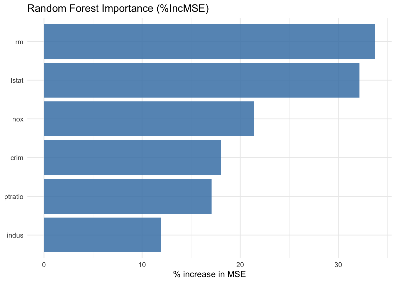
The randomForest object provides two common regression importance summaries, %IncMSE and IncNodePurity. We collect both to compare rankings.
This ranking is often informative, but it should not be treated as a fixed truth. Small rank changes can occur with different seeds, data splits, or hyperparameters.
14.6 Permutation Importance on Held Out Data
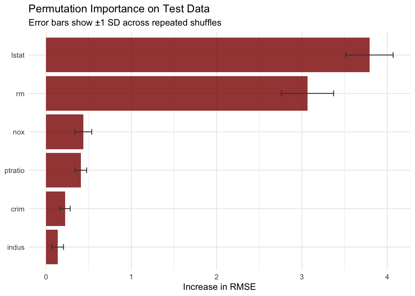
To complement model specific scores, we compute permutation importance directly on the test set with repeated shuffles.
perm_imp |>ggplot(aes(x =reorder(variable, mean_delta_rmse), y = mean_delta_rmse)) +geom_col(fill ="darkred", alpha =0.80) +geom_errorbar(aes(ymin = mean_delta_rmse - sd_delta_rmse,ymax = mean_delta_rmse + sd_delta_rmse ),width =0.15,color ="gray25" ) +coord_flip() +labs(title ="Permutation Importance on Test Data",subtitle ="Error bars show ±1 SD across repeated shuffles",x =NULL,y ="Increase in RMSE" ) +theme_minimal()
The dispersion bars help us avoid over interpreting very close ranks. If two variables have overlapping uncertainty ranges, it can be preferable to report them as similarly important rather than forcing a strict order.
14.7 Comparing Importance Definitions
A practical check is to compare rank agreement between methods.
High rank agreement can increase confidence that a variable is consistently influential under more than one definition. Disagreement is also informative, because it often signals correlation structure or interaction effects that deserve deeper inspection.
14.8 Correlated Predictors and Shared Signal
When predictors overlap strongly, attribution becomes ambiguous. We can diagnose this by inspecting the predictor correlation matrix.
If two variables are strongly correlated, shuffling one may have a limited effect because the other can partially recover the same information. In that case, a low marginal importance does not necessarily mean substantive irrelevance.
For communication, it is often helpful to pair feature importance with grouped interpretation, for example, discussing signal carried by related predictor families rather than only isolated variables.
14.9 From Ranking to Variable Selection
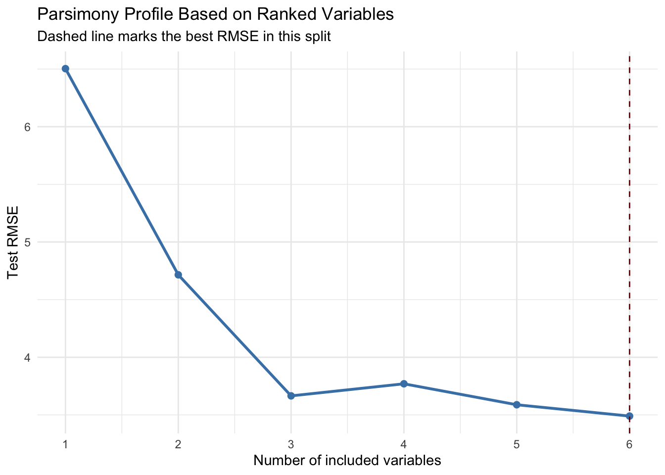
Importance ranking often motivates a second question, how many predictors do we need for a stable descriptive model? A simple approach is to order variables by importance, fit models with the top \(k\) variables, and inspect out of sample error as \(k\) grows.
best_k <- subset_perf$k[which.min(subset_perf$rmse)]subset_perf |>ggplot(aes(x = k, y = rmse)) +geom_line(color ="steelblue", linewidth =1) +geom_point(color ="steelblue", size =2) +geom_vline(xintercept = best_k, linetype ="dashed", color ="darkred") +scale_x_continuous(breaks =seq_len(length(ordered_vars))) +labs(title ="Parsimony Profile Based on Ranked Variables",subtitle ="Dashed line marks the best RMSE in this split",x ="Number of included variables",y ="Test RMSE" ) +theme_minimal()
This profile is intentionally pragmatic. It does not claim to identify a uniquely correct subset, but it helps us evaluate the trade off between parsimony and predictive adequacy in a transparent way.
14.10 A Brief Classification Illustration
Feature importance behaves similarly for classification, although impurity and loss definitions differ. We use the Pima diabetes data for a compact illustration.
Even in this short example, ranking should be interpreted jointly with domain context and class balance considerations. Importance identifies model reliance, not clinical causality.
14.11 Good Practice for Reporting Feature Importance
A careful descriptive report often benefits from a short checklist:
report which importance definition was used,
indicate whether evaluation is in sample, OOB, or held out,
include some notion of variability (for example repeated permutations),
note potential correlation induced dilution,
avoid causal language unless causal identification is justified separately.
These practices do not eliminate ambiguity, but they make interpretation more transparent and reproducible.
14.12 Summary and Key Takeaways
Feature importance is a global explanatory tool that ranks model reliance on predictors.
Impurity based and permutation based scores answer related but distinct questions, and both can be informative.
Correlated predictors can redistribute importance, so low marginal importance is not always low substantive relevance.
Ranking can guide variable selection through parsimony profiles that compare error across top \(k\) subsets.
Importance is descriptive unless paired with a separate causal design.
14.13 Looking Ahead
Feature importance tells us which predictors matter most for model performance, but it does not describe the functional shape of those effects. The next chapter therefore focuses on partial dependence and related profile methods, where we examine how predictions vary as individual predictors change across their observed ranges.
Fisher, Aaron, Cynthia Rudin, and Francesca Dominici. 2019. “All Models Are Wrong, but Many Are Useful: Learning a Variable’s Importance by Studying an Entire Class of Prediction Models Simultaneously.”Journal of Machine Learning Research 20 (177): 1–81. https://jmlr.org/papers/v20/18-760.html.